28. Electromagnetic radiation
28.1. Overview
Link to the program in this lesson:
Ever since Newton split sunlight into its component colors using a prism in the 1600s, physicists have been trying to explain the properties of light. This was a long debate, partly because the experimental evidence was confusing. Some of it suggested that light was made of particles, while others thought it was due to waves. This issue was not really settled until the 1920s, with the advent of quantum mechanics, where light has aspects of both particles and waves.
There is one aspect of this debate I want to focus on. Proponents of the wave theory had a serious question to confront: is light is a wave, what is waving? All other waves known at that time had a physical medium that oscillated – waves on the ocean are the motion of water, you hear sound waves because of vibrations of air. How do light waves reach the Earth from the Sun? There was a guess that there was a somewhat mysterious substance, called the “ether”, that filled all of space, whose vibrations were precisely light waves. Unfortunately, the ether theory had its own problems, and eventually, new experiments were done to show that the ether could not exist. For the most famous of these experiments, one of the two scientists involved was Albert Michelson, who served some time as instructor at the US Naval Academy; Michelson Hall is named after him! It was Einstein’s theory of special relativity, however, put the nail in the coffin for the ether.
In this lesson, we will explore the resolution of this problem. Spoiler alert: light doesn’t need anything to do the waving! Light is the arrangement of electric and magnetic fields in such a way that they self-propagate – light waves itself. The fact that light can do this is built into Maxwell’s equations of electromagnetism, one of the great triumphs of 19th century physics. What we will see in this lesson is that these equations are exactly what is needed. In particular, how the fields change in space leads to how they change in time; light is an electromagnetic wave where these two changes mutually reinforce each other to give a moving wave. We will see how this works using two of Maxwell’s equations: the Ampere-Maxwell law and Faraday’s law.
Here are the objectives for this lesson:
State the Ampere-Maxwell law and Faraday’s law.
State the speed of light in terms of the constants \(\mu_0, \epsilon_0\).
Describe the direction of travel for electromagnetic radiation in terms of its electric and magnetic fields.
28.2. Ampere’s circuital law
At the end of the last lesson, I motivated the equation giving the magnetic field due to a long, straight wire. To find this properly with the Biot-Savart law takes some effort, either with integral calculus, or else by using vPython to code an appropriate simulation. However, let’s take this relation as given; remember that the magnitude \(B\) of this field was
Based on this rule, we will find a relation that is much simpler to calculate, and can be used in a variety of situations. I will start with the long, straight wire, and imagine that I am moving in a circular path, whose center is at the center of the wire. Depending on how I walk around the circle, and which way the current is going through the wire, I will see the magnetic field either always in the same direction as I am walking, or else in the opposite direction. Below is a situation where the current is coming out directly towards you; we can use the right-hand rule to figure out the counterclockwise direction of the magnetic field created by this current.
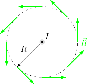
Fig. 28.1 Magnetic field vectors around path centered at current wire
I will now play a similar game to what I did in Lesson 27 to find the magnetic field at the center of a circular loop: namely, to approximate the circular path we are using here with a polygon. Suppose I am walking around the path in a counterclockwise direction. Then, I have a vector \(\Delta {\vec \ell}\) along each side of the polygonal approximation to the circular path. Notice this is much like what I did with the circular loop, but with one key difference. There, I used the \(\Delta {\vec \ell}\) to indicate the pieces of the current loop, whereas here, I am using it for the segments of the path where I measure the field due to the current wire at the center. The picture thus looks like that shown below. There are \(N = 12\) sides to the polygon approximation, and I have moved the magnetic field vectors \({\vec B}\) a short distance away from the wire for clarity.
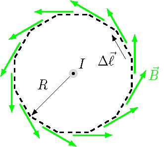
Fig. 28.2 Approximating the circular path with a polygon
The way I have drawn the vectors \({\vec B}\) and \(\Delta {\vec \ell}\), both point in the same direction. This means the angle between the two vectors is zero; therefore, for each segment, the scalar product is the product of their magnitudes:
Much like we did in Lesson 27, taking the limit as the number of polygon sides goes to infinity gives us the circumference of the original circular loop. Thus,
This shows us that, for this loop, Ampere’s circuital law works out. You can show that this law works for all cases with a collection of wires like this; you can think about what else you need to prove on a rainy day. However, we will see later in this lesson that Ampere’s circuital law is missing a crucial piece. It was Maxwell who noticed this, and completed the equation properly.
Problem
Write a vPython function circularLoopSum() which calculates the vector sum \(\sum_k {\vec B}_k \cdot \Delta {\vec \ell}_k\) along a circular loop, of radius \(R\), centered at a wire with current \(I\). Do this by approximating the circular loop as a polygon of \(N\) sides. The arguments of this function should be the radius R of the loop, the current I of the wire, and the number of sides \(N\) for the polygon. The function should return a scalar to represent the sum \(\sum_k {\vec B}_k \cdot \Delta {\vec \ell}_k\). It may be helpful to look back at the discussion in Lesson 27, and the function polyPerimeter() you had to write for a problem.
Answer: Here is a possible solution for the problem.
def circularLoopSum(R, I, N):

    # Definitions

    mu = 4 * pi * 1e-7           # Vacuum permeability (N / m)
    DQ = (2 * pi) / N            # Angle between adjacent points
    loop_sum = 0                 # Variable to store final sum

    # Calculate sum by looping over each segment

    for kkk in range(N):

        # Find line segment distance vector DL by
        # difference in r_{k + 1} - r_k

        DL = R * vector(cos((kkk + 1) * DQ), sin((kkk + 1) * DQ), 0) - \
             R * vector(cos(kkk * DQ), sin(kkk * DQ), 0)

        # Find magnetic field at angle halfway
        # between kkk * DQ and (kkk + 1) * DQ;
        # remember B is tangent to circle!

        B = (mu * I) / (2 * pi * R) * vector(-sin((kkk + 0.5) * DQ), cos((kkk + 0.5) * DQ), 0)

        # Take scalar product of these two vectors,
        # add this to sum

        loop_sum += dot(B, DL)

    # Return sum

    return loop_sum
Problem
Suppose there is a circular wire, with radius \(R\), and a uniform current \(I\) inside the wire. Use Ampere’s circuital law to find an algebraic equation for the magnitude \(B\) of the magnetic field at a distance \(r < R\) away from the center of the wire. Hint: What would be a good loop to use to solve this? How much current passes through this loop?
Answer: The magnitude \(B\) is given by
Notice that is matches the outside field magnitude at the boundary distance \(r = R\).
28.3. Non-conservative vector fields
Since this sum of scalar products will be important later, let’s play around with it a little. What precisely is it telling us? First, notice that it gave a non-zero answer for the magnetic field of a wire. To use a technical term, a “swirly” vector field will give some non-zero number for the sum. But doesn’t every vector field do the same thing? It turns out not. Here’s a simple example: suppose we look at the gravitational field \({\vec g}\) near the surface of the Earth, where \({\vec g} = (-g) {\hat y}\), and find the sum
around a square loop with sides of length \(L\), as shown below.
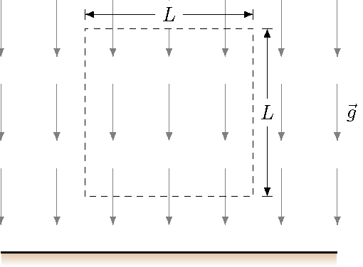
Fig. 28.3 Finding the sum of scalar products for the gravitational field
If we go around the loop in a counterclockwise direction, only two of the sides will give something other than zero for the scalar product, namely the two vertical sides. However, these will be opposite signs, and the sum is precisely zero.
I hope that there is a small bell ringing in your head, because this is very similar to what we did when we talked about conservative forces. In fact, this is exactly what is going on here: any “conservative” field will give a zero sum around a closed loop. By conservative field, I mean a field that would give rise to a conservative force, such as the forces of gravity or a spring. Much like those forces, a conservative field can be written in terms of a function, just like a conservative force can be derived from a potential energy, as in Lesson 20 (energy graphs). In particular, a conservative force \({\vec F}\) is the slope of a potential energy \(U_F\) vs. position \(r\) graph, with
Remember that we have defined fields from forces by dividing out by the appropriate physical quantity for the test object – the mass of a test mass for the gravitational field, and the charge of a test charge for the electric field. So a conservative field has a similar idea, and can be written in terms of a function much like the equation above. As an example, a conservative electric field is matched with the electric potential (or voltage) \(V\).
Non-zero sums for non-conservative fields
Given a closed loop made of distance vectors \(\Delta {\vec \ell}_k\) and a vector field \({\vec V}\) with values \({\vec V}_k\) at each segment of the loop, the sum
is non-zero only if the vector field \({\vec V}\) is a non-conservative field.
In three dimensions, every vector can be written in two pieces: the conservative part, and the non-conservative (or “swirly”) part. With a vector \({\vec V}\), the sum \(\sum_k {\vec V}_k \cdot \Delta {\vec \ell}_k\) around a closed loop only picks up the swirly piece. Now, when we found the electric field due to a point charge, in Lesson 25, this was a conservative field. Any collection of such charges will also give a conservative field. Another way I can describe these fields is Coulombic, because we derived the electric field for point charges from Coulomb’s law for the electrostatic force. Thus, any “swirly” or non-conservative electric field will also be non-Coulombic, i.e. not arising from a group of point charges.
Problem
Below is a list of fields \({\vec V}\) in a region of space. Find the sum \(\sum_k {\vec V} \cdot \Delta {\vec \ell}_k\) around the rectangular loop shown in the figure below. This sum has four terms, one for each side. To get a number for each term, evaluate the field at the center of each side, and take the scalar product of the distance vector along that side (going counterclockwise). You can find the distance vectors of the sides from the coordinates given for two of the rectangle’s corners. Which of the fields \({\vec V}_k\) are conservative fields?
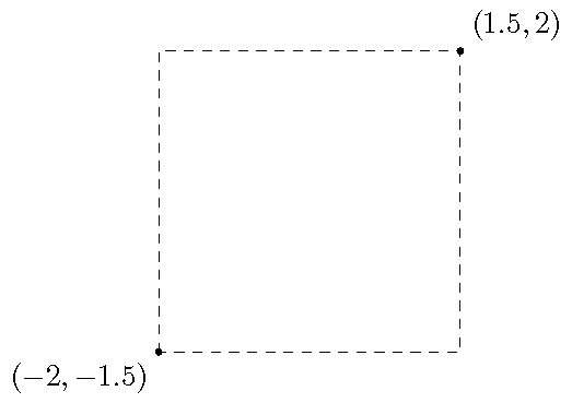
Fig. 28.4 Find the sum \(\sum_k {\vec V} \cdot \Delta {\vec \ell}_k\) using the centers of each side
\({\vec V}_1 = 2 {\hat x} - 7 {\hat y}\)
\({\vec V}_2 = -5 (r_x {\hat x} + r_y {\hat y})\)
\({\vec V}_3 = 3 (-r_y {\hat x} + r_x {\hat y})\)
\({\vec V}_4 = -4 \biggl[ \biggl( \frac{r_x}{r_x ^2 + r_y ^2} \biggr) {\hat x} + \biggl( \frac{r_y}{r_x ^2 + r_y ^2} \biggr) {\hat y} \biggr]\)
Answers: You should find the sum is zero for \({\vec V}_1, {\vec V}_2\), and \({\vec V}_4\); these are the conservative fields. The non-conservative field \({\vec V}_3\) gives a sum \(\sum_k {\vec V}_{3, k} \cdot \Delta {\vec \ell}_k = 73.5\).
Problem
Modify your vPython function circularLoopSum() from a previous problem, so it can calculate the sum of the scalar products around a circular loop of radius \(R\), for a particular vector field \({\vec V}\). Assume the circular loop is centered at the origin, and move around the loop in a counterclockwise fashion. Thus, the function now only needs two arguments: the radius R of the circular loop, and the number of polygon segments N to use in the calculation. The function will return a scalar which gives the sum \(\sum_k {\vec V}_k \cdot \Delta {\vec \ell}_k\) around the circular loop. Verify that the fields \({\vec V}_k\) from the last problem give either a zero or non-zero answer, based on whether you said the field was conservative or not.
It may be helpful to put the calculation for the vector field in a separate function calcField(), which you can call from the function circularLoopSum(). The function calcField() has a single argument, the position to calculate the field at, and it would return a vPython vector for the field \({\vec V}_k\) at that point.
Answer: First, here are the functions needs for each of the four given vector fields \({\vec V}_k\):
def calcFieldOne(pos):
    return vector(2, -7, 0)

def calcFieldTwo(pos):
    return -5 * vector(pos.x, pos.y, 0)

def calcFieldThree(pos):
    return 3 * vector(-pos.y, pos.x, 0)

def calcFieldFour(pos):
    return -4 * vector(pos.x, pos.y, 0) / (pos.x ** 2 + pos.y ** 2)
You can use these in the modified version of circularLoopSum() given below; you would have to modify each function above, so that it is called calcField().
def circularLoopSum(R, N):

    # Definitions

    DQ = (2 * pi) / N            # Angle between adjacent points
    loop_sum = 0                 # Variable to store final sum

    # Calculate sum by looping over each segment

    for kkk in range(N):

        # Find line segment distance vector DL by
        # difference in r_{k + 1} - r_k

        DL = R * vector(cos((kkk + 1) * DQ), sin((kkk + 1) * DQ), 0) - \
             R * vector(cos(kkk * DQ), sin(kkk * DQ), 0)

        # Find vector field at angle halfway
        # between kkk * DQ and (kkk + 1) * DQ;
        # notice the position is *not* the same
        # vector as the previous version of
        # this program, since it is a position,
        # not a tangent vector!

        field = calcField(R * vector(cos((kkk + 0.5) * DQ), sin((kkk + 0.5) * DQ), 0))

        # Take scalar product of these two vectors,
        # add this to sum

        loop_sum += dot(field, DL)

    # Return sum

    return loop_sum
For three of the four vector fields, you should get a number very close to zero, although not exactly, because of numerical errors (something like \(10^{-15}\) or so). Only for calcFieldThree() should you get a non-zero answer.
28.4. Electric and magnetic flux
We now need to take a detour and develop the idea of flux; we will use this to properly define the Ampere-Maxwell law and Faraday’s law later in this lesson. In particular, both of these laws deal with the change in a type of flux with time; one will deal with magnetic flux, the other with electric flux. For now, though, I will talk generically about “fields”, and then later apply it specifically to electric and magnetic fields.
Remember above that we found the scalar product of a field around a closed loop; what flux does is finds the amount of field going through the loop! Intuitively, we are counting the number of field lines that pass through the loop. If none of the field lines pass through the loop, then we should get zero flux. On the other hand, if the field lines pass straight through the loop, we should get maximum flux. This is shown pictorially below, where the closed loop is the dashed line, and the area enclosed by the loop is shaded in. The vector field \({\vec V}\) is represented by the arrows.
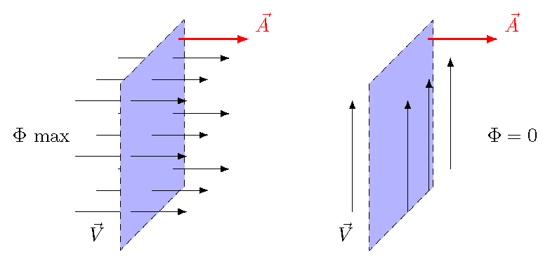
Fig. 28.5 Cases of maximum and minimum flux
Notice that in the picture above, I have put a vector \({\vec A}\) related to the area enclosed by the loop. This is the area vector \({\vec A}\) of this area; I wil come back to this vector later. For now, let’s see how our intuition for flux matches what is happening in the pictures. With maximum flux, we see this is when the vector field \({\vec V}\) through the area is in the same direction (or parallel) at the area vector \({\vec A}\). The flux is zero when \({\vec V}\) is perpendicular to \({\vec A}\) – the field is along the area, but not through it.
The words I am using here – “parallel” and “perpendicular” vectors – should get you thinking about the scalar product. This is exactly what we are going to use to find flux. Schematically, flux will be the scalar product \({\vec V} \cdot {\vec A}\) for the field \({\vec V}\) and area \({\vec A}\). So, all that’s left is to define the area vector. To do this, I first define the normal vector \({\hat n}\) for a given surface area to be a vector with unit magnitude that points perpendicular to the plane of the surface. Remember that “normal = perpendicular” in physics. Then, the area vector \({\vec A}\) of the surface is the vector \({\vec A} = A {\hat n}\) with a magnitude equal to the area \(A\) of the surface, and whose direction is given by the normal vector \({\hat n}\). An example of each of these vectors is shown below.
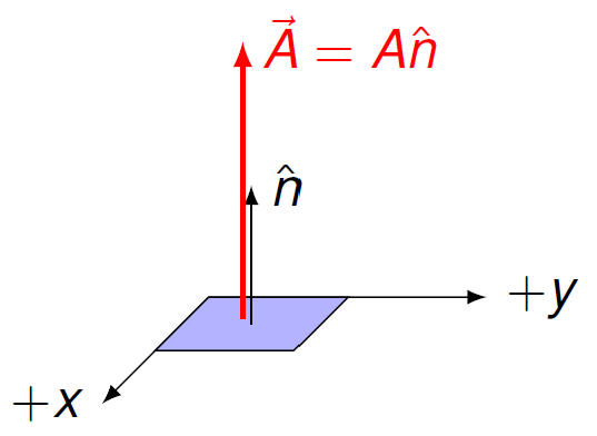
Fig. 28.6 Definition of the area vector
Problem
Suppose a cube with 10.0 cm sides is placed with its center at the origin, as in the figure below. Find the area vectors for each of the six sides of the cube, choosing their directions to point away from the cube’s center. Give the magnitudes of vectors in m\(^2\).
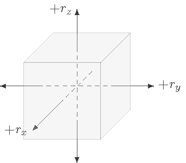
Fig. 28.7 Find the area vectors for each of the six cube faces
Answer: Since all of the cube’s faces have the same area of \(A = 10^{-2}\) m\(^2\) (not 1 m\(^2\) – watch your units!), the only important part is the direction of each area vector. These are as follows: \({\vec A}_{front} = A {\hat x}\), \({\vec A}_{back} = -{\vec A}_{front}\), \({\vec A}_{right} = A {\hat y}\), \({\vec A}_{left} = -{\vec A}_{right}\), and \({\vec A}_{top} = A {\hat z}\), \({\vec A}_{bottom} = -{\vec A}_{top}\).
For the moment, I have left the direction of the normal vector vague; after all, I could have it point in the opposite direction, and still be a normal vector. I will return to this point later in this lesson, when we get into Faraday’s law. At this point, let’s go ahead and define the fluxes for both electric and magnetic fields; obviously, the definitions will be very similar.
Quantity: electric flux
Symbol: \(\Phi_E\) (“phi sub E”)
Definition: For an electric field \({\vec E}\) passing through a surface with an area vector \({\vec A}\), the electric flux is given by
Units: N m\(^2\) / C
Strictly speaking, this definition should include the fact that the electric field \({\vec E}\) is constant over the area \({\vec A}\); if it is not, then the electric flux would instead be found by dividing the area into smaller pieces, then add up the electric fluxes through each piece \({\vec A}_k\) due to the electric field \({\vec E}_k\), that is
For a general application, this is how you will use electric flux (and the same for magnetic flux), but I will generally just use constant fields for this lesson.
The definition of magnetic flux is basically the same, although its units have their own name, unlike the electric flux!
Quantity: magnetic flux
Symbol: \(\Phi_B\)
Definition: For a magnetic field \({\vec B}\) passing through a surface with an area vector \({\vec A}\), the magnetic flux is given by
Units: webers (Wb) = T \(\cdot \)m\(^2\)
Problem
The magnetic field through the circular area (\(r = 13.0\) cm) shown below points into the page and has an initial value of 150 mT. This field decreases in magnitude at a rate of 17.0 mT/s. The normal vector is chosen to point out of the page. Based on the information given, what is the magnetic flux (in mWb) through the circle? Be sure to include the appropriate sign.
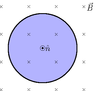
Fig. 28.8 Changing magnetic field through a circular loop
Answer: \(-7.96\) mWb
What will be important for both the Ampere-Maxwell law and Faraday’s law is not so much the flux itself, but instead the change in flux with time. Thinking in terms of the vectors associated with \(\Phi\), this can happen for two basic reasons. If the field vector \({\vec B}\) is changing, then the change in flux \(\Phi_B\) with time is given by
Notice that \({\vec B}\) and \(\Delta {\vec B} / \Delta t\) can have either the same or opposite direction. If the size of the field is increasing, they will have the same direction; if the magnitude is decreasing, they are in the opposite direction. A side view of the vectors, and their changes in time, is illustrated below. The same story can happen with the electric field \({\vec E}\) as well.
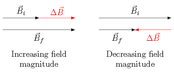
Fig. 28.9 The field, versus its change in time
On the other hand, the flux can vary if the area vector is changing as well; in this case,
Here, the area vector can change either because the size of the loop is changing, or else because the normal vector is changing in direction (i.e. imagine a rotating loop of wire). Of course, there is also the possibility that both vectors are changing with time! In addition, the angle between the vectors is changing, but this can only happen if one or both vectors vary with time.
Problem
Use Figure 28.8 for this problem as well. The magnetic field through the circular area (\(r = 13.0\) cm) shown above points into the page and has an initial value of 150 mT. This field decreases in magnitude at a rate of 17.0 mT/s. The normal vector is chosen to point out of the page. Based on the information given, what is the rate of change in the magnetic flux (in \(\mu\)Wb/s) through the circle? Be sure to include the appropriate sign.
Answer: \(+902 \ \mu\)Wb/s
Problem
The graph shows the change in the \(x\) component of an electric field as a function of time. Suppose you are measuring this electric field through a square loop, with 35.0 cm sides, and choosing the normal vector \({\hat n}\) of the loop to be in the \(+x\) direction. Find the size of the electric flux (in N m\(^2\) / C), and the change in the electric flux (in N m\(^2\) / C s), at each of the times listed below.
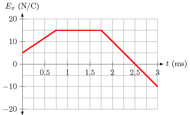
Fig. 28.10 Graph of the electric field component \(E_x\) vs. time \(t\)
0.500 ms
1.50 ms
2.50 ms
Answers: (1) \(\Phi_E = 1.43\) N m\(^2\)/C and \(\Delta \Phi_E / \Delta t = 1.63 \times 10^3\) N m\(^2\) / C s; (2) \(\Phi_E = 1.84\) N m\(^2\)/C and \(\Delta \Phi_E / \Delta t = 0.00\) N m\(^2\) / C s; (3) \(\Phi_E = 0.00\) N m\(^2\)/C and \(\Delta \Phi_E / \Delta t = -2.45 \times 10^3\) N m\(^2\) / C s
28.5. Faraday’s law
Let’s now put some of these ideas into practice, and turn to the first of the two Maxwell’s equations we will be using, namely Faraday’s law. I want to recap the pieces we will use in this relation. First, remember we talked about the sum of scalar products \(\sum_k {\vec V}_k \cdot \Delta {\vec \ell}_k\) of a vector field \({\vec V}\) around a closed loop, given by the distance vectors \(\Delta {\vec \ell}_k\). This sum is non-zero only when the vector field is non-conservative, i.e. the vector field is “swirly”. For Faraday’s law, we will be considering the electric field around the loop, so it will be testing for non-conservative electric fields. We can use the same closed loop to find the magnetic flux \(\Phi_B\) through the loop. However, the important aspect will be the change in this magnetic flux with time; Faraday’s law relates this change to the scalar product sum.
Faraday’s law
Suppose you have a closed loop, which is the boundary of an area \(A\). The loop is made up of segments \(\Delta \ell_k\), each with its own distance vector \(\Delta {\vec \ell}_k\). Faraday’s law says that a non-conservative electric field gives rise to a change in the magnetic flux through the area \(A\). This relation is given by
To give you some context, as I mentioned briefly above, the (conservative) electric field \({\vec E}\) is related to the voltage difference \(\Delta V\) along any path (not just closed!) by the scalar product sum along the path. Thus, the quantity
is a voltage difference, just like you have for a battery. So, Faraday’s law says that any voltage difference around a closed loop gives rise to a change in magnetic flux. A conserative electric field will always have zero voltage difference around a closed loop; this is how I originally defined a conservative field! So only non-conservative (or “swirly”) electric fields will result in a magnetic flux changing with time.
Here’s an important point you should keep in mind: the cause of a voltage difference around a closed loop will result in an effect of a changing magnetic flux with time. Unfortunately, Faraday’s law is not usually taught in this manner, but is described with the cause being the change in magnetic flux, and the result is the non-conservative electric field. However, this does not make any sense. Let’s go back to Newton’s second law, written in terms of linear momentum \({\vec p}\) as
Hopefully it makes sense to say that the net force is the cause of the change \(\Delta {\vec p}\) in linear momentum, rather than the other way around! We have seen many equations of this form, where the rate of change of one physical quantity is given in terms of the values of other quantities. For all of these, we say that the rate of change is a result, rather than why things happen.
Now, let’s turn back to something I mentioned before, about the direction of the normal vector we use to define the magnetic flux. There is also another choice we have to make, namely how we go around the closed loop at the outside of the area. It turns out that, for Faraday’s law to be consistent, we need to link these choices together! If we do this properly, it doesn’t matter which way I go around the loop, as long as I pick the normal vector to match my choice. Using Faraday’s law correctly depends on the consistency of these two choices.
So how does this work? Consider the area shown below, where I have drawn arrows on the boundary loop to indicate the direction I will go around this loop. Now, curl the fingers of your right hand around the boundary loop; your thumb should naturally point in the direction I have drawn the normal vector \({\hat n}\). Said a different way, for the choice of normal vector given, the positive direction around the loop will be in the counterclockwise direction. For Faraday’s law to be consistent, you must make the choice of loop direction and normal vector match up like this. Since the area vector \({\vec A}\) is just a scalar multiple of the normal vector \({\hat n}\), this gives the relationship between the area vector \({\vec A}\) and the positive direction along the boundary.
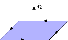
Fig. 28.11 Relationship between the area vector and the positive direction along the surface boundary
Problem
The magnetic field through the circular area (\(r = 13.0\) cm) shown in Figure 28.8 points into the page and has an initial value of 150 mT. This field decreases in magnitude at a rate of 17.0 mT/s. The normal vector is chosen to point out of the page. Based on the information given, which way is the positive direction around the boundary of the circle?
clockwise
counterclockwise
into the page
left
out of the page
right
Answer: The positive direction around the circle boundary is counterclockwise.
Let’s now put together the pieces for the magnetic field through the circular area, that you have been working through with some of the last few problems. In particular, we can see how to use Faraday’s law in this situation. Since the magnetic flux is changing through the loop, Faraday’s law tells us that this is the result of a non-conservative electric field \({\vec E}\). Since the magnetic field is uniform, this electric field will have circular field lines, as shown below; I will show after the picture why the direction of the field is chosen the way it is.
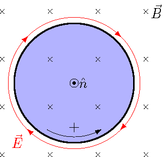
Fig. 28.12 Non-conservative electric field causing the decreasing magnetic field
From the last problem, the choice of the normal vector gives that the positive direction around the loop is counterclockwise; this is indicated on the diagram above as a reminder. This will be the direction of the vectors \(\Delta {\vec \ell}_k\) we use in the sum \(\sum_k {\vec E} \cdot \Delta {\vec \ell}_k\). Thus, this is just like the vPython function circularLoopSum() you wrote for an earlier problem; we can imagine approximating the circular loop as a polygon, like we did there. Now, let’s turn to the left-hand side of Faraday’s law. Even though the magnetic field \({\vec B}\) is into the picture, opposite the direction of the normal vector \({\hat n}\), the field is decreasing in size. Therefore, the vector \(\Delta {\vec B} / \Delta t\) points out of the picture, in the same direction as the normal vector. This is how, in a previous problem, you found the change in flux \(\Delta \Phi_B / \Delta t\) with time to be positive. Bringing all of this together, we have that the left-hand side of Faraday’s law is positive, thus so must the right. Because of the minus sign, this means that the sums of the scalar products \({\vec E}_k \cdot \Delta {\vec \ell}_k\) are negative. This is how I know the direction of the non-conservative electric field above.
Finally, let’s find the magnitude \(E\) of this electric field; it will be constant in size, since the magnetic field is also uniform. Thus, using the circumference of the loop, we have that
The minus sign went away, since the scalar products were all negative (i.e. there is a \(\theta = 180.^\circ\) angle between each \({\vec E}_l\) and \(\Delta {\vec \ell}_k\) in the sum). Solving for the electric field magnitude \(E\) using Faraday’s law, we get
From the earlier problem, we know all of these values, so we get an electric field magnitude \(E\) of 1.11 mN/C.
Problem
The figure below shows two circular regions, where \(R_1 = 30.0\) cm and \(R_2 = 25.0\) cm; in each region, there is a uniform magnetic field, while there is no magnetic field outside the regions. The magnetic field in region 1 has a magnitude of \(B_1 = 65.0\) mT, while that in region 2 has a size \(B_2 = 80.0\) mT; the directions of the fields are those shown in the diagram. Both fields are decreasing at a rate of 9.30 mT/s. For each of the three labeled paths, find the sum \(\sum_k {\vec E}_k \cdot \Delta {\vec \ell}_k\) (in units of N m / C) around the path. Use a counterclockwise direction to go around each path.
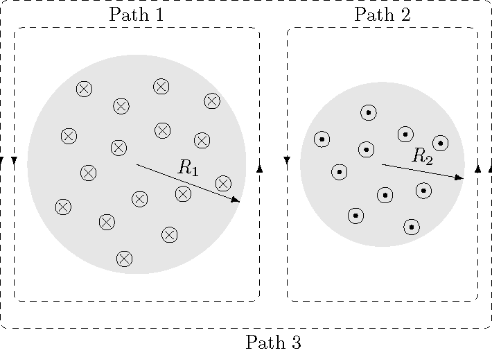
Fig. 28.13 Find the sum \(\sum_k {\vec E}_k \cdot \Delta {\vec \ell}_k\) around each labeled path
Answers: \(-2.63 \times 10^{-3}\) N m / C (path 1); \(+1.83 \times 10^{-3}\) N m / C (path 2); \(-8.04 \times 10^{-4}\) N m / C (path 3)
28.6. The Ampere-Maxwell law
I started with lesson with Ampere’s circuital law, which relates the current wire passing through a closed loop to the scalar product using the wire’s magnetic field. However, there is a problem with this equation: it only works in the situation where there is no change. The standard explanation of this problem is to imagine two uncharged metal plates (these form a circuit element known as a capacitor), which are then connected using wires to a battery. The battery will cause charge to flow through the wires, so that one plate has its excess electrons pulled off, moved through the wires and battery, to be deposited on the other plate. Thus, the net result of connecting the plates to the battery is an increasing positive charge on one plate, and an increasing negative charge on the other. A side view of the situation is represented in the picture below.
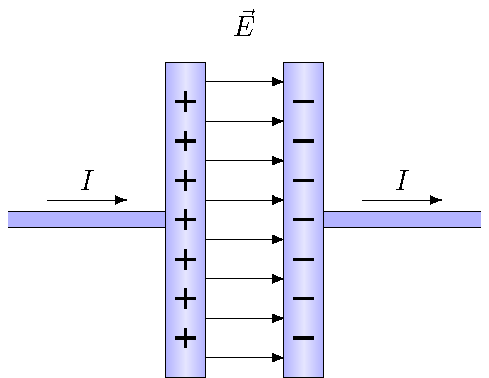
Fig. 28.14 Charging plates connected by wires
Now, suppose we are near one of the wires, but far away from the charging plates. Using Ampere’s circuital law, we see that the current through the wire is creating a magnetic field around the wire. So far, so good. If we look at a point between the two plates, the two plates have opposite charges, so there is an electric field between the two plates. Since the plates are charging, this electric field between the two plates is increasing in magnitude.
What I said above for the loop around the wire made an assumption about what area I used for that loop, namely, the area was like a soap bubble, so that it was as small as possible. This is the situation shown to the left in the figure below. But that’s not the only way I can draw the area. In fact, as long as the loop used is the boundary of the area, I can use any area I want. So let’s try an area which passes between the plates, as shown on the right; this area is like a hat or an open soup can, where the wire is passing into the open side. This is where the problem comes in – the wire no longer goes through the shaded area! According to the circuital law, this would imply that there is no magnetic field around the loop now, since there is no current going through the area, as drawn on the right-hand side.
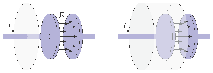
Fig. 28.15 Two possible areas for the same closed loop
Maxwell was the one that resolved this issue, by pointing out that, even though there is no enclosed current for this way of drawing the area, there is a changing electric field through the area. This means the area, drawn on the right-hand side of the figure, has a changing electric flux through it. So to get everything to work out, we just need to this changing flux in the equation. If you work out how this is done, you will get the Ampere-Maxwell law, as written out below.
The Ampere-Maxwell law
Suppose you have a closed loop, which is the boundary of an area \(A\). As before, the loop is made of segments \(\Delta \ell_k\), each with its own distance vector \(\Delta {\vec \ell}_k\). The Ampere-Maxwell law states that the electric flux through the area \(A\) can change from two causes, an unbalanced change in the magnetic field around \(L\), and a non-zero current passing through the area \(A\).
The constant \(\epsilon_0\) is the vacuum permeability, and is related to the Coulomb constant \(k\) by \(\epsilon_0 = 1/(4 \pi k)\). Thus, with \(k = 8.99 \times 10^9\) N m\(^2\) / C\(^2\), then \(\epsilon_0 = 8.854 \times 10^{-12}\) C\(^2\) / N m\(^2\).
The right-hand side of this equation is just what we had with Ampere’s circuital law. When there is no changing electric flux through the area, these two terms still balance out, as that law stated. Notice that we need a changing \(\Phi_E\), since a constant electric current through a wire would generate a constant electric flux. There was only a problem in the situation above when the plates were charging.
Problem
Suppose you turn on the lamp by your bed, and 15.0 amperes of current instantly flows through the 14-gauge wire (which has a diameter of 1.63 mm) from the wall outlet to the lamp. Assume that the magnetic field created by the current is zero at a particular moment. What size is the rate of change of the electric field (in N / C s) through the wire, due to the current?
Answer: \(\Delta E / \Delta t = 8.12 \times 10^{17}\) N / C s (this rate is very rapid, which is why the electric and magnetic fields from such a current wire are essentially formed instantaneously)
28.7. Electromagnetic waves
Now we will pull everything else in this lesson together, and construct a light wave, based on the Ampere-Maxwell and Faraday laws. The basic picture of what is happening is shown below: perpendicular, oscillating electric and magnetic fields are combined together in such a way, so that the wave continues to move at a constant speed in the \(+z\) direction. The figure shows the fields at a particular instant of time, with the electric field \({\vec E}\) oscillating along the \(x\) axis, and the magnetic field \({\vec B}\) along the \(y\) axis. As time moves forward, the peaks and troughs of the wave will move towards increasing \(z\).
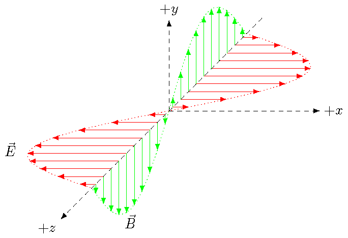
Fig. 28.16 Electric and magnetic fields of a light wave at a particular instant of time
Although it may not be obvious from the picture, what I am doing is assuming that the electric and magnetic fields only depend on the \(r_z\) and \(t\) values; in other words, the fields at points which differ only in the \(r_x\) or \(r_y\) coordinate are the same. This is why I have only shown how the fields change along the \(z\) axis. This greatly simplifies the analysis we will do, since I don’t have to worry about changes in \(r_x\) or \(r_y\). This type of wave is known as a plane wave; it is a good description of light waves coming from the Sun and hitting the Earth.
Since I will eventually code this into a vPython program, I only define the electric and magnetic fields at certain points, indexed by \(k\), and separated by a spatial interval \(\Delta r_z\). As we will see later, this is a lot like the time interval \(\Delta t\) we have been using in programs throughout the course.
Because of the way the two fields are changing in time, they reinforce each other in exactly the right way for this to happen. Let’s set up how these fields can propagate themselves, without the need for any kind of physical medium. I will first look at using Faraday’s law, using the setup shown in the next figure. Here, we are looking down the \(y\) axis, with the \(+x\) axis towards the top of the figure. Thus, the magnetic field \({\vec B}\) is pointing either into or out of the picture, while the electric field \({\vec E}\) points towards the top or bottom.
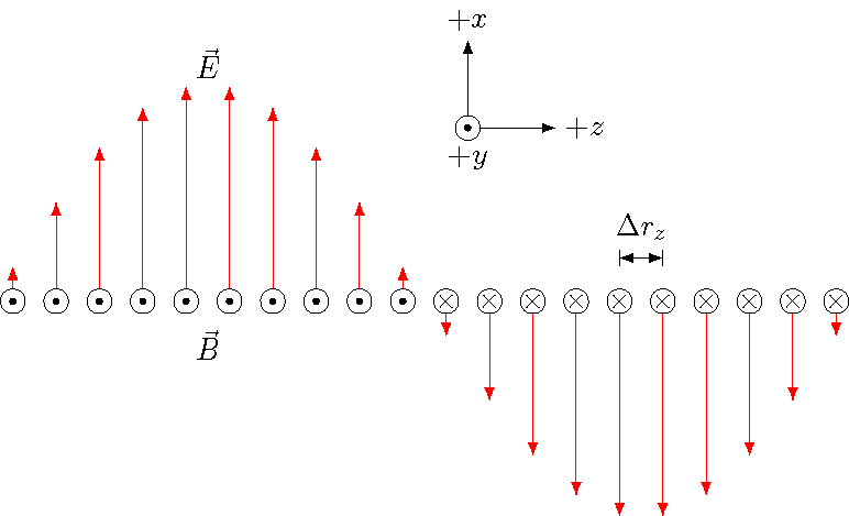
Fig. 28.17 Looking along the magnetic field vectors at the electromagnetic wave
Now, for Faraday’s law, we have to relate the sum \(\sum_k {\vec E}_k \cdot \Delta {\vec \ell}_k\) of scalar products around a loop, to the change in the magnetic flux \(\Phi_B\) through that loop. So obviously, we need to pick a good loop! I will do that as shown in the picture below, where I have focused on a particular part of the wave. The loop I am using here is centered at the point \(k\) where I measure the magnetic field \({\vec B}_k\), and has sides \(2 \Delta r_z\) (i.e. twice the separation between the field points). I chose this, because now I can use the electric fields at the neighboring points \(k - 1\) and \(k + 1\) to find the sum \(\sum_k {\vec E}_k \cdot \Delta {\vec \ell}_k\). In particular, since the field points along the \(x\) axis, I only need the scalar products along the left and right sides of the loop.
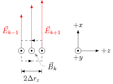
Fig. 28.18 Using Faraday’s law for a loop in the field
Thus, going around the loop in a counterclockwise direction, the sum of the scalar products for the loop shown is
On the other side of Faraday’s law, we need to find the change in the magnetic flux through the loop. Remember that magnetic flux \(\Phi_B\) is the scalar product of the magnetic field through the loop, and the area vector of the loop. The area vector is made of the loop’s area, which here is \((2 \Delta r_z)^2\), multiplied by the normal vector \({\hat y}\). Putting this together gives
Here, I have pulled out the constant area and time interval, leaving just the change \(\Delta B_{k, y}\) in the \(y\) component of the magnetic field. This change is in time, so \(\Delta B_{k, y}\) represents the final minus initial values of \(B_{k, y}\). I want to put these last two equations together into Faraday’s law; however, before I write it in the form we will use to update the magnetic field in time, let me show it as given below. What I have done is moved all of the spatial intervals \(\Delta r_z\) to one side of the equation, and kept the time interval to the other. This gives
Remember the minus sign out front on the right side of the equation comes from Faraday’s law!
If you’re familar with differential calculus, this form should look familiar. If I take both limits \(\Delta t, \Delta r_z \to 0\), then Faraday’s law says that the derivative of \(B_y\) in time is equal to the negative of the \(z\) derivative of \(E_x\). Thus, changes in the electric field as position changes give rise to changes in the magnetic field with time. It is exactly this relationship which gives rise to the wave behavior of light.
Let’s now keep going, and get an equation more helpful for updating in a vPython program. I will drop the \(x\) and \(y\) subscripts, since the these components just give the magnitudes of each field, so I can emphasize the initial and final values for the vectors. Then, we have the equation above is
This gives the field magnitude \(B_{k, f}\) at point \(k\) after a time interval \(\Delta t\), based on the original values of the electric and magnetic fields at the previous time.
Next, we do a similar process to find the change in the electric field \({\vec E}\) with time, using the Ampere-Maxwell law. The picture below is a rotated version of the previous one; notice that the \(+x\) axis now point into the picture, while the \(+y\) axis points towards the top. However, the spacing \(\Delta r_z\) between field points is the same. I use a loop similar to the one we used before.
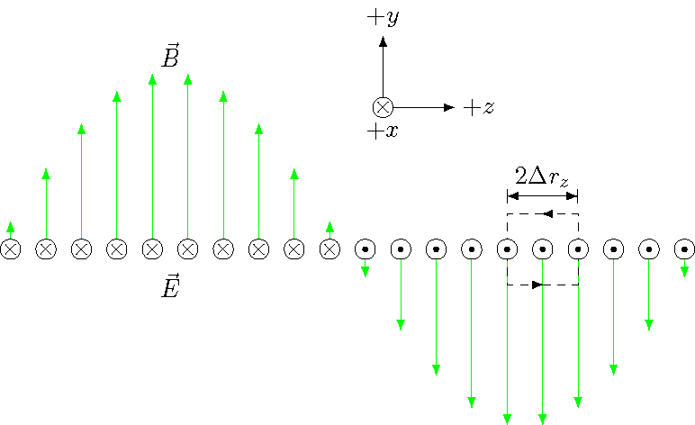
Fig. 28.19 Looking along the electric field vectors at the electromagnetic wave
There is no current within the loop, so that part of the Ampere-Maxwell law is zero. The rest follows what we did above, with the sum of the scalar products
and the change in electric flux,
There is one slight change here, because of how the coordinate axes are now placed; since we went counterclockwise around the loop, the normal vector is \(-{\hat x}\), not \({\hat x}\). This is why there is a net minus sign in the last step above. Finally, using the Ampere-Maxwell law, we get a very similar equation to what we had above, just switching the electric and magnetic fields:
These equations are in the program below. Running the program may help understand how the equations are actually working, which I talk about below the app.
So what are these equations telling us? If we look at the first one, it says that if the electric field magnitude increase with the index \(k\) (i.e. increases with increasing \(r_z\)), then the magnetic field magnitude \(B_k\) will decrease with time. On the other hand, if the electric field magnitude decreases with larger \(k\), then the magnetic field is increasing in size. This may seem backwards, but it is exactly what we need to have a wave move in the \(+z\) direction, or to the right in the pictures above. If you look at the right-hand side of one of the crests, then you want the magnetic field to increase as the crest is moving towards you (from the left); the field gets bigger as the crest comes from the left to the location you are looking at. If you are at the left-hand side of a crest, the field should be getting smaller, as the crest moves away from you, to the right.
The discussion above focused on the change in the magnetic field with time, but because the equations are essentially the same, the electric field will change in time the same way. The only real difference between the two equations is the constant \(1 / (\mu_0 \epsilon_0)\); although I will not show it here, it turns out this gives the speed of the wave! If I denote the speed of light as \(c\), then
To sum up, we have seen how the Ampere-Maxwell law and Faraday’s law work together to give combinations of electric and magnetic fields that move through space at a fixed speed of light. This was a pretty amazing discovery, tying together a lot of different phenomena into a single description! It also led to a revolution in technology, as our understanding of electromagnetic fields allows the development of many different devices.
Problem
In the program above, the electric and magnetic fields are given as arrow objects, each with a given pos and axis, in the lists E_array and B_array, respectively. You can change their initial properties in these lists. What happens if you flip the starting directions of just one of the fields? Does it matter which field you flip? What happens if you flip the direction of both fields?
Answer: If you flip the direction of only one field, regardless of which one it is, the wave will travel in the opposite direction, namely the \(-z\) direction. Flipping both fields restores the direction of the electromagnetic wave as the \(+z\) direction.
The results of the last problem can be summarized by saying that the electromagnetic wave travels in the direction of the vector product \({\vec E} \times {\vec B}\) of the two fields. In the program above, \({\vec E}\) is along the \(x\) axis, \({\vec B}\) is along the \(y\) axis, giving \({\vec E} \times {\vec B}\) in the \(+z\) direction at every point of the wave. Although I will not show it here, it turns out we can go further, and assign meaning to this vector product.
Poynting vector
The Poynting vector \({\vec S}\) is a vector defined by
The magnitude of the vector at any point gives the rate of change of energy flux for the electromagnetic field; its direction gives the direction of motion for the electromagnetic wave. The units of \({\vec S}\) are J/s m\(^2\).
28.8. Summary
This lesson shows how electric and magnetic fields are really unified in a single idea called electromagnetism. As we saw, this is because Maxwell’s equations tell us that if there is a non-conservative field of one type, that will lead to a change in flux for the other. For example, Faraday’s law says that, if there is a non-conservative electric field around a closed loop, then there is a change in magnetic flux through the loop. The Ampere-Maxwell law says the same for a non-conservative magnetic field giving a changing electric flux. So, note the causation: one kind of non-oonservative field causes the other to change with time. This matches how we have talked about relations with quantities changing in time throughout the year.
This relationship between electric and magnetic fields is exactly what is necessary to have electromagnetic waves, combinations of oscillating electric and magnetic fields that propagate at a fixed speed. In fact, the constants \(\mu_0\) and \(\epsilon_0\) in the equations gives exactly what this speed is! All electromagnetic waves will travel with this fixed speed \(c\). Knowing the speed of light is constant throughout the Universe was a big conceptual leap for physics, and led directly to Einstein’s theory of special relativity. More broadly, the roadmap provided by Maxwell’s equations was eventually used as a guide to explain other fundamental forces in the Universe, such as the strong and weak nuclear forces, using a quantum mechanical framework. Unfortunately, the same is not yet true about gravitation, but this is an active area of research.
To sum up, what is presented in this lesson is just the tip of a broad area of physics, but the concepts here are deep and powerful ones. Hopefully, this brief overview gives you some idea of these basic ideas. And this summit of physics is a good place to end the class!
After this lesson, you should be able to:
Define conservative and non-conservative fields.
Use the Ampere-Maxwell and Faraday laws to calculate the change in electric or magnetic flux, due to the appropriate non-conservative field.
Describe how electric and magnetic fields combine to give propagating waves.