.ipynb .pdf

Binder

Contents

2. Vectors and vPython

2.1. Overview

Links to programs in this lesson:

1. Yellow arrow

2. createTriad()

3. scalarMult()

4. twoVectorSum()

5. Graphical vector addition

This lesson covers two crucial portions of the class: the mathematical idea of a vector, and the programming tool called vPython. Let’s briefly summarize each of these in turn.

The intuitive idea you should have for a vector is an arrow – something with a direction, and a size or scale. On the other hand, scalars are basically numbers, with no direction associated with them. Many of the physical quantities we will talk about in physics are best described as vectors, such as velocities, forces, momenta, and fields. You will see vector equations that relate these quantities. However, it is important to realize that these equations have a few important differences with equations made up only of scalars. Understanding these differences is crucial for a good grasp of physics concepts, so we will continually revisit this topic over the course of many lessons.

There are many ways to describe a vector, and this lesson will hopefully give you a handle on these. First, you can go back to the idea of a vector as an arrow, and draw these on paper to see how to add or subtract them. This will be the idea behind “graphical vector addition”. This technique is great for giving you a rough idea of the size and direction of a vector. We will use graphical vector addition frequently in this context – for example, when we draw the “free body diagram” of the forces acting on an object in Lesson 13 (Solving force problems). We will also draw the “vector diagram” of many vectors, in order to find their “vector components”. This is the second, and more mathematical, way of describing vectors. The components of a vector tell you how much of the vector is along each axis. This will also allow you to calculate the sum of multiple vectors. As a way to tie these two methods together, you will also see how to draw vectors using programming techniques. In particular, you will see that the codes using the mathematical relations gives you the graphical addition of arrows we would expect.

To help understand these and many other physics concepts, we will use the vPython package. Often in a programming language, the command of the language must be supplemented to make more features available. The 3D graphics package vPython for the Python programming language was created by David Scherer while he was a student at Carnegie Mellon University. It has since been modified and developed by many others into a vibrant community. vPython allows you to create and animate 3D objects, and to navigate around in a 3D scene by spinning and zooming, using the mouse. vPython will build upon your new Python programming experience, and hopefully you will have fun doing so!

So why do we need vPython? Why can’t we just use the formulas and calculate things with them? My experience as a teacher is that many times, students see mathematical equations as a fancy machine that you put numbers into, then you get other numbers out of. What do they mean? “Well, my roommate (or a supplemental instructor, or somebody in my platoon) told me to do it this way, and…” This means you don’t really get it at all. Learning is doing. Full stop. My goal with using vPython is that you understand physics a little better than you did when started the class.

How to read these lessons

This is the first lesson where we start dealing with calculations of physical quantities. I emphasized at the beginning of Lesson 01 that these lessons are meant to be interactive, and it is the same here: do not read these notes like a novel. What I mean by that is

• You should have a pencil, paper, and a calculator by your side before you even start reading the lesson.

• As you go through, try the problems listed, and check to see if you can do them. If not, come to class with a question about your confusion.

• Don’t skip parts just because you don’t understand them! Make a decent effort to carefully read the text, and try the problems. Note this does not mean to get bogged down. If you devote a good deal of time, and it still does not make sense, come and ask me, either in class or EI. But at least give it the ol’ college try.

I will confess that I often don’t follow my own advice, and I frequently come to regret it. I can get away with it when reading about material I already understand fairly well, but when I am trying to learn something new, I usually crash and burn because I have not been methodically working through the concepts. Then I have to start over, and read it again. And again. And again. If learning was easy, everybody would do it.

Here are the objectives for this lesson:

• Describe the difference between a scalar and a vector.

• Describe the effect of scalar multiplication of a vector.

• Write a vector in proper unit vector form, given its components.

• Add together multiple vectors graphically.

• Add together multiple vectors in unit vector form.

• Create a vPython object, and set its attributes.

2.2. Vectors

2.2.1. Scalars and vectors

Throughout the lessons of this class, there will be links to simulations that others have created and placed on their websites. One good source for many of these is PhET Interactive Simulations site; I will refer to these simulations as “PhETs”. If you go to the site, you’ll notice there are simulations in other subject besides physics. To start off, the following PhET may be helpful as you work through this lesson. It allows you to play around with vectors, and illustrates many of the concepts discussed in this lesson. The application below has several parts:

• “Explore 1D” – Here, you can add up to three vectors, either all along the \(x\) axis, or all along the \(y\) axis. You can stretch or shrink the vectors, and see how the vector sum changes.

• “Explore 2D” – This is the same idea in two dimensions. Here, for all the vectors (including the vector sum), you can see either magnitude and direction of each vector, or else the \(x\) and \(y\) vector components, represented in different ways for each vector.

• “Lab” – Add up as many vectors of the same color as you wish. Each of the individual vectors can be changed in magnitude and direction by clicking and dragging the vector.

• “Equations” – Experiment with various vector equations, given at the top of the screen, relating three vectors \({\vec a}, {\vec b}\), and \({\vec c}\). Change the size of the vectors by selecting “Base Vectors” on the side.

Now let’s get into the nitty gritty, and talk about scalars vs. vectors. Many of the things we do in physics will depend on the idea of a “vector”, so it is very important to understand the difference between a vector and a “scalar”. Intuitively, a scalar is just a number. If we put units on a scalar, some examples would be the time of day you are reading this, and the temperature in the room where you are reading it. A vector, on the other hand, can be best thought of as an arrow – a vector is a quantity that has both magnitude (size) and direction. The velocity of an object is a vector, since it has a size (how fast are you moving?) and a direction (which way are you moving?).

To sum up, there are two basic mathematical quantities we will use this year in physics class:

1. Scalar: A number representing the size (or magnitude) of a quantity. Examples are mass, temperature, electric charge.

2. Vector: Intuitively, we can think of a vector as an arrow, which has both size and direction. Examples include velocity, acceleration, force.

Whenever you see a symbol with an arrow sign above it, you should read it as a vector. Examples are the velocity vector \({\vec v}\) and the acceleration vector \({\vec a}\). A symbol without an arrow sign is a scalar. Note that there is a scalar associated with every vector – namely, its size! So, when I talk about the momentum vector, I use the symbol \({\vec p}\), but when I talk about the scalar magnitude of the momentum vector, I use \(p\) (or sometimes \(|{\vec p}|\)). Know the difference!

2.2.2. Scalar multiplication

I will now draw representations of vectors as arrows. Each arrow will point in the same direction as the vector, and I will scale the arrow to show the size of the vector. It is this last part you have to be careful about – many different kinds of quantities are vectors, so don’t get too wrapped up in the idea of “magnitude = length”. This is why I used the word scale before. I can draw an arrow to represent a force vector, where 1 centimeter of arrow length on my drawing denotes 10.0 N of force magnitude.

Vectors are not just distances

The reason I emphasize this here is that sometimes you will draw multiple vectors – representing different quantities – in the same problem, and if you confuse every vector with a length (or each other!), you will have problems. One place I see this a lot is when doing projectile motion problems (Lesson 07). Here, you may have an initial velocity vector to show how a cannonball is launched from a cannon, and a displacement vector giving its final position relative to its start. These vectors are not the same! They are generally not in the same direction, either. However, I sometimes see students calculate the final position of a cannonball using the initial velocity. Projectiles do not move in straight lines, because of the gravitational field of the Earth. Confusing your vectors will lead to this false conclusion.

Vectors can be multiplied by a scalar, which you can think about as “stretching” the vector if the scalar is positive, along with flipping the vector’s direction if the scalar is negative. Thus, scalar multiplication can either change the size of the vector

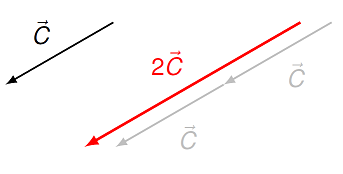
Fig. 2.1 Scalar multiplication by a positive scalar

or change the direction by reversing its direction.

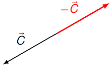
Fig. 2.2 Multiplying a vector by \(-1\)

In the first figure, the size of the vector \(2 {\vec C}\) is twice that of the original vector \({\vec C}\), but the direction is unchanged; in the second, \(-{\vec C}\) has the same length as \({\vec C}\), but opposite direction.

You will see many examples of such scalar multiplication of vectors in physics. In Lesson 03 (velocity and the Euler method), for example, you will see this with the definition of average velocity:

\[ {\vec v}_{avg} = \frac{\Delta {\vec r}}{\Delta t} \]

Here, \(\Delta {\vec r}\) is the vector change in position (called the displacement vector), while \(\Delta t\) is the scalar change in time. This is just scalar multiplication in disguise, since

\[ {\vec v}_{avg} = \biggl( \frac{1}{\Delta t} \biggr) (\Delta {\vec r}) \]

Thus, the average velocity vector is found by scalar multiplication of the displacement vector \({\vec r}\) by the scalar \((1 / \Delta t)\); the average velocity of an object is just the displacement of the object rescaled.

2.2.3. Vector addition

We wil often add vectors together; for example, we will see in Lesson 11, with Newton’s laws of motion, that the acceleration of an object depends on the vector sum of all the forces acting on it. Pictorially, vectors are added by placing them “head” (or “tip”) to “tail”. To get the vector \({\vec A} + {\vec B}\):

• Draw the first vector, \({\vec A}\)

• Draw the second vector, \({\vec B}\), with the tail of \({\vec B}\) at the tip of \({\vec A}\)

• The resultant vector \({\vec A} + {\vec B}\) is drawn from the tail of \({\vec A}\) to the tip of \({\vec B}\)

• Note the order we add the vectors doesn’t matter!

Moving vectors

Notice that we can pick up and move vectors around, as long as we don’t change their scale or direction! You often need to do this when using graphical vector addition.

An example of this process is shown in the figure below.

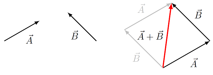
Fig. 2.3 Adding two vectors graphically

Problem

Based on the figure below, which of the following vector equations is correct?

1. \({\vec M} + {\vec N} = {\vec S}\)

2. \({\vec M} + {\vec N} = {\vec T}\)

3. \({\vec M} + {\vec T} = {\vec N}\)

4. \({\vec S} + {\vec T} = {\vec M}\)

5. \({\vec S} + {\vec T} = {\vec N}\)

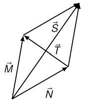
Fig. 2.4 Adding two vectors graphically

Answer: The correct answer is \({\vec M} + {\vec N} = {\vec S}\). Notice you can “pick up” \({\vec N}\) and move it to the top of the picture, as long as it points in the same direction and has the same length. Then, you would start at the tail of \({\vec M}\) (which is at the same point as the tail of \({\vec S}\)), travel to its tip, which is now at the tail of \({\vec N}\). Finally, moving to the tip of \({\vec N}\), you also arrive at the tip of \({\vec S}\), so the vector equation is satisfied.

Just like vector addition, we will frequently subtract vectors as well. In fact, you will see this often, starting in Lesson 03, where the operation of “difference” (or \(\Delta\)) is defined. Thus, finding the average displacement means subtracting the initial position \({\vec r}_i\) from the final position \({\vec r}_f\). Vector subtraction can be rewritten as vector addition.

\[ {\vec A} - {\vec B} = {\vec A} + (-{\vec B}) \]

To get the vector \({\vec A} - {\vec B}\):

• Draw the first vector, \({\vec A}\)

• Draw the second vector, \({\vec B}\), with reversed direction to make it negative, with the tail of \(-{\vec B}\) at the tip of \({\vec A}\)

• The resultant vector \({\vec A} - {\vec B}\) is drawn from the tail of \({\vec A}\) to the tip of \(-{\vec B}\)

This process is shown in the figure below.

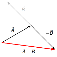
Fig. 2.5 Subtracting two vectors graphically

Problem

Based on the figure below, how would you express the red vector \({\vec T}\) in terms of the vectors \({\vec M}\) and \({\vec N}\)?

1. \({\vec M} + {\vec N} = {\vec T}\)

2. \({\vec M} - {\vec N} = {\vec T}\)

3. \({\vec N} - {\vec M} = {\vec T}\)

4. \({\vec M} = {\vec T}\)

5. \({\vec N} = {\vec T}\)

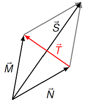
Fig. 2.6 What is the correct vector equation for \({\vec T}\)?

Answer: The correct answer is \({\vec M} - {\vec N} = {\vec T}\). Notice that one way to see this is to add the vector \({\vec N}\) to both sides of the equation, giving \({\vec M} = {\vec N} + {\vec T}\). By using the tip-to-tail method outlined above, you can see this is a correct vector equation. Adding and subtracting vectors in a vector equation is an acceptable mathematical operation, just like it is for scalars.

Hopefully you find the graphical representation of vectors to be helpful. I often will draw the vectors when working on a problem, just as a double-check to make sure my answers make sense. As mentioned earlier, this will also be part of the problem-solving procedure we use many times throughout the year, such as with forces and Newton’s 2nd law, or when adding electric field vectors together. Getting into the habit of having this thought process in the back of your head is a handy way of avoiding egregious mistakes.

2.2.4. Unit vector notation

Drawing vectors as arrows can be helpful, but it is not the entire method. To get accurate results, we need to bring mathematical calculations into the picture. This will be done using “vector components”, which uniquely give a vector in terms of a list of numbers. This method is powerful, and reflects a quantum leap in the study of science that started with the ideas of Rene Descartes in the 17th century.

As a way of introducing vector components, we will first give a brief history of the grid system of Manhattan. In 1811, a commission established a grid pattern for future roads built on Manhattan island, with avenues running roughly north-south, and streets going east-west. This urban plan helped New York City deal with its exponential growth in population during the 19th century; the five boroughs together were the largest city in the US by 1835. If we ignore some of the rough spots in the grid (due to either history, or living on an island that is not exactly a rectangle!), you can give the position of any street in Manhattan by two numbers: street and avenue. Throw in a height, and you have three numbers giving any spot in the island’s airspace.

Fig. 2.7 The Commissioners Map of the City of New York, 1807 (source)

Suppose we start in front of the Guggenheim Museum (5th Ave & 88th St) and walk to the Chrysler Building (3rd Ave & 43rd St). Then, you sneak up to the 70th floor to see the gymnasium. How can we describe the walk from start to finish? No matter how you do it, you have gone back two avenues, down 45 streets, up 70 floors. This is your displacement vector, which we will define more formally in Lesson 03. For now this is the straight-line vector between your starting and ending points, and is independent of the path you actually take. The idea behind unit vector notation is to uniquely describe a vector in a series of numbers, as done with trips in Manhattan; these numbers are called vector components.

There are several ways to mathematically describe a vector. For now, we use unit vector notation, which lists how much of a vector is along each of the three coordinate axes \(x, y\) and \(z\). You can see how this notation is related to the vector \({\vec A}\) in Figure 2.8 . In unit vector notation, this vector is written as

\[ {\vec A} = A_x {\hat x} + A_y {\hat y} + A_z {\hat z} \]

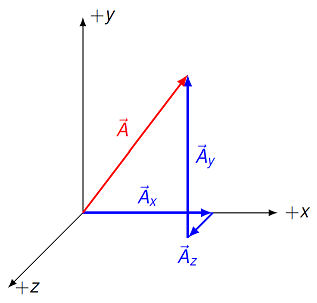
Fig. 2.8 Dividing a generic vector into three component vectors

The three scalars \(A_x, A_y,\) and \(A_z\) are the vector components of the vector \({\vec A}\). The directions are given by the three “unit vectors” \({\hat x}, {\hat y},\) and \({\hat z}\). The vector \({\hat x}\) is a vector of size 1 (“unit” size) that points in the \(+x\) direction. Similarly, \({\hat y}\) points in the \(+y\) direction and \({\hat z}\) points in the \(+z\) direction, both with size 1. If \({\hat x}\) has a size of 1 and points in the \(+x\) direction, then \(3 {\hat x}\) also points in the \(+x\) direction but has size of 3, and \(-2 {\hat x}\) has size of 2, but points in the \(-x\) direction. We will introduce unit vectors more formally in Lesson 07 (vector magnitude and direction).

2.3. vPython

2.3.1. Your first vPython object

The last picture above may be a little confusing, since it is a flat representation of a three-dimensional object. To get a better feel for vectors, it is time to learn about the vPython package, and use it to create arrows to represent vectors. As mentioned at the beginning of this lesson, vPython allows you to create and animate 3D objects, and to navigate around in a 3D scene by spinning and zooming, using the mouse. If you go to the site vpython.org, you can find examples and documentation that may be helpful; a quick introduction is also available.

Python vs. vPython

If you pay attention, you will notice I say “Python” when referring to the programming language, and “vPython” when I start talking about creating visual simulations. One advantage of using either of the sites Glowscript.org or Trinket.io is that we don’t have to worry too much about the difference between Python and vPython. Since vPython is added on to Python, anything that works in Python will work in vPython.

However, if you create a new Trinket using an account on that website, make sure that you select “Glowscript” when you want to create a program with vPython in it. This will be the same as if you are using an account on Glowscript.org, just with a different user interface. Also, when you create a new Glowscript Trinket, you have two options of how you write the program. I will always use the “Python” option, and I recommend you do, too. This will get you used to writing code as it appears in these lessons.

Whenever you create visual simulations in vPython, you are creating objects. In many programming languages, special types of procedures and functions are created that exhibit a given list of properties, or attributes. The first vPython object we will use is arrow, and just like the names says, this will be a representation of an arrow. Its possible attributes include its position, length, direction, and color. As you go through this lesson, you will create arrow objects to show various aspects of vector math. So let’s get started! The program below tells the computer to create an arrow. Run the program, then we will talk about what it is doing in detail.

Back to program list

This program creates an object A which is a vPython arrow. We will get back to its attributes in a moment, but let’s first talk about how to play around with our first vPython object. After you run the program, and get the resulting arrow in the right-hand window, hold down both mouse buttons, and then move the mouse on this scene. You should see that you are able to zoom the arrow into and out. Now try holding down only the right mouse button, then move the mouse. You should find that you are able to rotate around the arrow, because of the change in the sphere’s shading; vPython is creating a light source at a specific point which is illuminating the sphere. Note that you are changing your viewpoint (like moving a camera) rather than changing the position of the sphere. You are zooming and rotating the camera, not the sphere.

Now back to the arrow and the attributes it was assigned. Its position A.pos is the origin, or the vector <0, 0, 0>.

Object attributes

If I have an object object with attribute attribute, then I refer to the attribute of the object as object.attribute. As we will see later, this is exactly how vPython uses it as well, so if we want to change the value of the attribute, this is how we will do so in the code.

Here, I am using an alternative method of showing the vectors, which is what vPython uses itself. The vector <-2, 3, 0>, for example, is the same thing as the vector

\[ -2 {\hat x} + 3 {\hat y} + 0 {\hat z} \]

in unit vector notation. If you ever print out a vector in vPython, the result will be three numbers (in \(x, y, z\) order) with the angled brackets, so I wanted you to know how to map this over to unit vector notation.

Back to positions and axes. The position of the tail of a vector A in vPython is given by A.pos. The attribute A.axis describes how to get to the tip of the vector, when starting from the tail. Thus, the three-dimensional position of the tip of the vector is the vector sum A.pos + A.axis.

Fig. 2.9 Finding the location of the tip of an arrow object in vPython

This is an key conceptual point, so let’s write it out mathematically, just to make sure you get the idea. There is a special point called the “origin”, which has coordinate \((0, 0, 0)\). The tail of the arrow (i.e. the point A.pos) will have a position vector \({\vec r}_{tail}\) given relative to the origin; the same thing is true for the tip of the arrow, with position \({\vec r}_{tip}\). Then the arrow object A in vPython represents the mathematical vector \({\vec A}\), so that starting from the tail and moving along \({\vec A}\), you reach the tip. As an equation, this says

\[ {\vec r}_{tail} + {\vec A} = {\vec r}_{tip} \]

In other words, starting at the origin, moving to the tail, and then moving along the vector \({\vec A}\), is exactly the same as if you start from the origin and move straight to the arrow’s tip. Written another way, the vector \({\vec A}\) is just the difference between the tip and tail position vectors, or

\[ {\vec A} = {\vec r}_{tip} - {\vec r}_{tail} \]

We are going to see variations of this equation throughout the year, so I emphasize it now. This is an example of the vector differences we saw earlier in this lesson.

Continuing on, the object A has two other attributes. Hopefully A.color is obvious, but note the way it is defined: not color = yellow, but color = color.yellow. More importantly, we have given the size and direction of the arrow as the attribute A.axis. This gives the vector components of the arrow object, which way it points starting from the tail at A.pos. Think of these numbers as the streets, avenues, and heights of the Manhattan example.

When you are looking at an object created in vPython (before you move it around as described above), there are specific directions for each of the three coordinate axes \(x, y\), and \(z\). Specifically, the \(+x\) axis points to the right of the screen, the \(+y\) axis points towards the top of the screen, and the \(+z\) axis points out of the screen, directly towards you. The three negative axes point in the opposite directions to those just described. These axes are shown in the figure below.

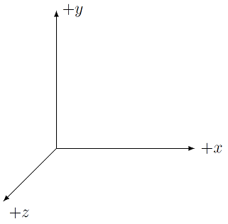
Fig. 2.10 Coordinate axes in vPython

The program below gives a three-dimensional representation of the coordinate axes in vPython. The procedure createTriad() creates arrows xArr, yArr, and zArr, each pointing with length 1 along one of the coordinate axes.

Variable names

The names of the variables used in functions do not have to be the same as those given to the returned variables. It may be useful to actually call them something different, so you know when you are using which one.

Back to program list

Thus, the length and direction of the arrow A from the previous program are described by its three vector components in A.axis: 2 units to the right (\(+x\) direction), 3 units upward (\(+y\) direction), and 1 unit “into” the screen (\(-z\) direction). For the example given above, where you traveled from the Guggenheim Museum to the Chrysler Building gymnasium, we could write the total trip as

\[ {\vec A} = (-2 \ \text{ave.}) {\hat x} + (-45 \ \text{st.}) {\hat y} + (+70 \ \text{fl.}) {\hat z} \]

Notice that this is just a combination of scalar multiplication for each of the three terms, along with a vector sum of the pieces along each axis. Thus, we can think of the vector \({\vec A}\) as the sum of three vectors: \(A_x {\hat x}\) in the \(\pm x\) direction, \(A_y {\hat y}\) in the \(\pm y\) direction, and \(A_z {\hat z}\) in the \(\pm z\) direction. So, speaking figuratively, you first “move” an amount \(A_x\) along the \(x\) axis, then an amount \(A_y\) on the \(y\) axis, and finally \(A_z\) along the \(z\) axis.

Problem

Which of the following correctly illustrates the \(x\) and \(y\) components of vector \({\vec A}\)?

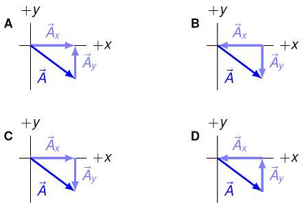
Fig. 2.11 Combining graphical vector addition with the components of unit vector notation

Answer: Remember that vector addition is always tip-to-tail. Since we are adding together \({\vec A}_x = A_x {\hat x}\) and \({\vec A}_y = A_y {\hat y}\) to get the total vector \({\vec A}\), then the tails of \({\vec A}\) and \({\vec A}_x\) must be at the same point, and similarly for the tips of \({\vec A}\) and \({\vec A}_y\). Thus, the correct answer is \(C\).

Problem:

A person’s velocity \({\vec v}\) is 4.00 m/s in the north direction, 7.00 m/s in the east direction, and 2.50 m/s straight down. How would you express the velocity in unit vector notation? Select the correct choice below.

1. \({\vec v} = (4.00\ \textrm{m/s}) {\hat x} + (7.00\ \textrm{m/s}) {\hat y} + (2.50 \ \textrm{m/s}) {\hat z}\)

2. \({\vec v} = (7.00\ \textrm{m/s}) {\hat x} + (4.00\ \textrm{m/s}) {\hat y} + (-2.50 \ \textrm{m/s}) {\hat z}\)

3. \({\vec v} = (7.00\ \textrm{m/s}) {\hat x} + (11.0\ \textrm{m/s}) {\hat y} + (2.50 \ \textrm{m/s}) {\hat z}\)

4. \({\vec v} = (11.00\ \textrm{m/s}) {\hat x} + (4.00\ \textrm{m/s}) {\hat y} + (-2.50 \ \textrm{m/s}) {\hat z}\)

Answer: The usual convention is that east is in the \(+x\) direction, and \(+y\) direction is taken to be north, if we are looking down at the ground. Note this would mean that up is the \(+z\) direction! Using this convention, then the correct answer is \({\vec v} = (7.00\ \textrm{m/s}) {\hat x} + (4.00\ \textrm{m/s}) {\hat y} + (-2.50 \ \textrm{m/s}) {\hat z}\), since downward is in the \(-z\) direction.

Now, suppose we start with the resultant vector from the last question,

\[ {\vec v} = (7.00\ \textrm{m/s}) {\hat x} + (4.00\ \textrm{m/s}) {\hat y} + (-2.50 \ \textrm{m/s}) {\hat z} \]

In vPython, this vector would be defined (and then printed out) by

v = vector(7.00, 4.00, -2.50)
print(v)

Thus, the components are listed in the usual order \(x, y, z\). As mentioned previously, if you ran this two-line program, vPython would print out the vector v as <7, 4, -2.5>.

2.3.2. Scalar multiplication with vector components

Now, let’s see how scalar multiplication and vector addition works when we use numerical vector components. In fact, we have already been doing this! The vector \(2 {\hat x}\) simply takes the vector \({\hat x}\) pointing in the \(+x\) direction with a length of 1, and multiplies it by 2.

Here is slightly more involved example.

Problem

Given the vector \({\vec A}\) below, what is the unit vector notation for the vector \({\vec B} = 4{\vec A}\)?

\[ {\vec A} = 2 {\hat x} + 3 {\hat y} - {\hat z} \]

Instead of giving the answer here, let’s do the same operation in vPython, and see how it works. You can then verify your answer to the previous problem! The function scalarMult() below takes the arguments k and vec. The function then multiplies the scalar k by the vector A to get a new vector k * A, which is what it returns. After you have solved the problem above, run the program below to confirm your answer.

Notice the way that this scalar multiplication is done, by increasing the size of A.axis. Remember that A.axis is the attribute that determines how long the vector is, and which direction it points, using a vPython vector. If you change the size of all the vector components of A.axis by scalar multiplication, the arrow will change size by the same scale. This is different than A.pos, which determines the position of the arrow’s tail.

Back to program list

Problem

In Lesson 25, you will see the concept of an electric field. Suppose you have a charged particle with charge \(q\) (units of coulombs, or “C”) placed in an electric field \({\vec E}\) (units of newtons/coulomb, or “N/C”). Then the electrostatic force \({\vec F}_e\) (units of newtons, or “N”) on the charge, due to this field, will be

\[ {\vec F}_e = q {\vec E} \]

This is just scalar multiplication, as we have just discussed.

1. Assume that a charge is \(+2.50\) C is placed in an electric field given by \({\vec E} = (-5.25 \textrm{ N/C}) {\hat x} + (1.40 \textrm{ N/C}) {\hat y} + (3.75 \textrm{ N/C}) {\hat z}\). What is the electrostatic force \({\vec F}_e\) on the charge, in unit vector notation? Be sure to include the proper units!

2. Use the same electric field as the previous problem, but now assume that the charge is \(-17.3\) C. What is the electrostatic force \({\vec F}_e\) on the charge, in unit vector notation?

Answers:

1. \({\vec F}_e = (-13.1 \textrm{ N}) {\hat x} + (3.50 \textrm{ N}) {\hat y} + (9.38 \textrm{ N}) {\hat z}\)

2. \({\vec F}_e = (90.8 \textrm{ N}) {\hat x} + (-24.2 \textrm{ N}) {\hat y} + (-64.9 \textrm{ N}) {\hat z}\)

Vectors are not scalars

It is vitally important that you do not confuse the scalar multiplication of vectors with the multiplication of two scalars! Do not confuse multiplying two scalars (\(6 = 2 \times 3\)) with the scalar multiplication of a scalar and a vector (\({\vec B} = k{\vec A}\)). They use the same symbol *, but mean two different things! If you are not careful about this, you can create errors in your Python code. For example, if you multiply two scalars, but vPython is expecting a vector, an error will be reported.

Later in Lesson 13, I will introduce the scalar product, a mathematical operation where you take two vectors and get a scalar. Again, this is not multiplication, in the sense that you multiply two like objects, and get another one back. It is also different in that there are many vector pairs whose scalar product is zero!

The gist of all this is you have to think about vectors differently than “ordinary” numbers, or scalars. Starting to do this now will save you a lot of grief down the road. This is why we use different notation: \(A\) is a scalar, \({\vec A}\) is a vector.

Note, though, that its size has increased in every direction – it is twice as thick as well! To avoid this issue for very long vectors, we can set the arrow attribute shaftwidth. Then only the vector’s length changes with changing axis, but not its width. An example of this is shown in the code below, comparing two arrows with the same length, but different shaftwidths.

arrow(pos = vector(0, 0.5, 0), axis = vector(2, 0, 0))
arrow(pos = vector(0, -0.5, 0), axis = vector(2, 0, 0), shaftwidth = 0.1)

Try these commands in a vPython program; the positions of the arrows are shifted, so you can more easily see the difference between the objects. This shift is accomplished by using the attribute pos in the lines defining the two vectors.

To sum up, here is a list of all the attributes you have covered for arrow objects.

Attribute	Description
axis	Vector from tail to tip of arrow (vector)
color	Arrow color (color.xxx or vector)
pos	Position of arrow tail (vector)
shaftwidth	Determines arrow thickness (scalar)

Fig. 2.12 The various attributes defining an arrow object in vPython

2.4. Vector addition

2.4.1. Using unit vector notation

Now that we have discussed both unit vector notation (one way to mathematically represent a vector), and drawn arrows to show vectors in vPython, let’s go back to Manhattan, so we can start talking about how to add multiple vectors. Consider the following situation:

1. For a weekend trip, you take the train from RI into Penn Station (7th Av. and 31st St.)

2. From there, you walk to Times Square (7th Av. and 44th St.)

3. Finally, you meet a friend in front of the NY Public Library (5th Av. and 41st St.) for a hot dog and drink

4. What is the total displacement in terms of streets and avenues?

We can add up the changes in streets and avenues for each leg as shown in the table below.

Trip	Change in avenues	Change in streets
Penn Station \(\to\) Times Square	0	+ 13
Times Square \(\to\) NY Public Library	-2	-3
Total	-2	+ 10

Notice what we have done here. Since avenues and streets are perpendicular, moving along a street only changes which avenue I am on, and vice versa. So, to find the total change in position, I can add the change in avenues first, then separately add the change in streets. These two numbers represent your displacement. This is why vector components are so powerful: whatever I do, I do them separately to the \(x\) components, then to the \(y\) components (and possibly the \(z\), if they are there!), to get my final vector. This is because the \(x, y\), and \(z\) axes are all perpendicular – moving along one of the axes does not change the values along the other two. If I represent my first vector as

\[ \Delta{\vec r}_1 = (0 \ \text{ave.}) {\hat x} + (13 \ \text{st.}) {\hat y} \]

and my second as

\[ \Delta{\vec r}_2 = (-2 \ \text{ave.}) {\hat x} + (-3 \ \text{st.}) {\hat y} \]

then the vector sum \(\Delta {\vec r} = \Delta {\vec r}_1 + \Delta {\vec r}_2\) is

\[ \Delta {\vec r} = \Delta r_x {\hat x} + \Delta r_y {\hat y} = (\Delta r_{1, x} + \Delta r_{2, x}) {\hat x} + (\Delta r_{1, y} + \Delta r_{2, y}) {\hat y} = (-2 \ \text{ave.}) {\hat x} + (10 \ \text{st.}) {\hat y} \]

Problem

Given two acceleration vectors (in units of centimeters per second squared, or “cm/s\(^2\)”)

\[ {\vec a}_1 = (6.20\ \textrm{cm/s}^2) {\hat x} + (-7.11 \ \textrm{cm/s}^2) {\hat y} + (2.63\ \textrm{cm/s}^2) {\hat z} \]

\[ {\vec a}_2 = (-4.42\ \textrm{cm/s}^2) {\hat x} + (-3.25 \ \textrm{cm/s}^2) {\hat y} + (1.91\ \textrm{cm/s}^2) {\hat z} \]

what is the resultant vector \({\vec a}_{tot} = {\vec a}_1 + {\vec a}_2\)?

1. \((-10.6\ \textrm{cm/s}^2) {\hat x} + (-3.86 \ \textrm{cm/s}^2) {\hat y} + (4.54\ \textrm{cm/s}^2) {\hat z}\)

2. \((1.78\ \textrm{cm/s}^2) {\hat x} + (-3.86 \ \textrm{cm/s}^2) {\hat y} + (0.720\ \textrm{cm/s}^2) {\hat z}\)

3. \((1.78\ \textrm{cm/s}^2) {\hat x} + (-10.4 \ \textrm{cm/s}^2) {\hat y} + (4.54\ \textrm{cm/s}^2) {\hat z}\)

4. \((10.6\ \textrm{cm/s}^2) {\hat x} + (10.4 \ \textrm{cm/s}^2) {\hat y} + (-0.720\ \textrm{cm/s}^2) {\hat z}\)

5. \((10.6\ \textrm{cm/s}^2) {\hat x} + (-3.86 \ \textrm{cm/s}^2) {\hat y} + (0.720\ \textrm{cm/s}^2) {\hat z}\)

Answer: \({\vec a}_{tot} = (1.78\ \textrm{cm/s}^2) {\hat x} + (-10.4 \ \textrm{cm/s}^2) {\hat y} + (4.54\ \textrm{cm/s}^2) {\hat z}\)

The next problem features solving for an unknown vector, starting from a vector equation. If you use addition and subtraction of vectors, you can solve this just like you would a scalar equation. However, you can not multiply or divide vectors!

Problem

Suppose you have two force vectors \({\vec F}_A\) and \({\vec F}_B\), such that

\[ {\vec F}_A + {\vec F}_B = {\vec F}_{net} \]

In addition, you know that

\[ {\vec F}_A = (-9.15\ \textrm{N}) {\hat x} + (4.77 \ \textrm{N}) {\hat y} + (-1.38\ \textrm{N}) {\hat z} \]

\[ {\vec F}_{net} = (-6.92\ \textrm{N}) {\hat x} + (3.36 \ \textrm{N}) {\hat y} + (5.01\ \textrm{N}) {\hat z} \]

What is the vector \({\vec F}_B\) (in N) in unit vector notation?

Answer: \({\vec F}_B = (2.23\ \textrm{N}) {\hat x} + (-1.41 \ \textrm{N}) {\hat y} + (6.39\ \textrm{N}) {\hat z}\)

2.4.2. Vector sums in vPython

Let’s go back to calculating the sum of vectors using vPython. Suppose we are given the vectors

\[ {\vec A} = 2 {\hat x} + 3{\vec y} - {\hat z} \qquad {\vec B} = -4 {\hat x} + {\vec y} + 5{\hat z} \]

and we want to find the vector sum \({\vec C} = {\vec A} + {\vec B}\). In vPython, the code for this is in the next program. First, try calculating the result yourself, then run the program below and check to see if the computer prints out the answer you expect.

Back to program list

Problem

Using the vectors \({\vec A}\) and \({\vec B}\) defined above, find \(-{\vec A}\) and \({\vec A} - 2 {\vec B}\).

Answers: \(-{\vec A} = -2 {\hat x} - 3{\vec y} + {\hat z}\); \({\vec A} - 2{\vec B} = 10 {\hat x} + {\vec y} - 11{\hat z}\).

Problem

Write a vPython procedure signFlip() that takes a vPython vector A as an argument, representing the vector \({\vec A}\), and returns the vPython vector equivalent to the vector \(-{\vec A}\).

Answer: Here is a simple implementation of signFlip().

def signFlip(A):
    return -A

Problem

Write a vPython procedure vectorMath() that takes two vPython vectors A and B, representing the vectors \({\vec A}\) and \({\vec B}\), and returns the vPython vector equivalent to \({\vec A} - 2{\vec B}\).

Answer: One possible program is given below.

def vectorMath(A, B):
    return A - 2 * B

2.4.3. Showing vector sums with arrows

Now, let’s look at how to show graphical vector addition in vPython. We will create arrow objects representing the vectors, then create a third arrow to give their vector sum. First, running the program below shows the original two vectors aVect and bVect.

Back to program list

Next, we want to add these two vectors together. When we created the vectors, their tails were both at the same location, so we need to move one of the vectors so that its tail is at the tip of the other. Beneath the lines already given in the program above, type in the code

bVect.pos = aVect.pos + aVect.axis

to move the tail of B to the tip of A. This changes bVect.pos so that the tail of vector \({\vec B}\) is moved to the tail of vector \({\vec A}\), then along the vector \({\vec A}\) itself until it is at the tip of \({\vec A}\), as described above. Run the program again to make sure this looks right.

Problem

Create a third arrow rVect that represents the vector sum of the previous two vectors, that is, \({\vec R} = {\vec A} + {\vec B}\). The tail of \({\vec R}\) should be at the tail of \({\vec A}\), so define rVect.pos = aVect.pos. The tip of \({\vec R}\) should be at the tip of \({\vec B}\), so the axis of rVect should be equal to the axes of the two vectors \({\vec A}\) and \({\vec B}\) – this moves the tip of \({\vec R}\) along \({\vec A}\) and then along \({\vec B}\). Print out the components of the vectors rVect, by removing the # in front of the print statement at the end of the program. Run the program to verify that the graphical vector addition is correct.

Answer: Here is a way to complete the program.

# Create arrow rVect representing vector sum
# R = A + B

rVect = arrow(pos = aVect.pos, axis = aVect.axis + bVect.axis, \
              color = color.red, shaftwidth = 0.1)

Note that we could have done it the other way around, so that we move the tail of \({\vec R}\) to the tail of \({\vec B}\) and then add the two axes together to move the tip of \({\vec R}\) to the tip of \({\vec A}\).

Problem

Change the program above to complete the graphical vector addition as described above. Specifically, the tail of aVect must now be moved to the tip of bVect. Then, the tail of rVect will be at the tail of bVect, while the tip of rVect is at the tip of aVect.

Answer: Here is the complete program you should have, so that the graphical vector addition is done using the method described in the problem.

# Create two vectors A and B

aVect = arrow(axis = vector(2, 2, -1), color = color.green, \
              shaftwidth = 0.1)
bVect = arrow(axis = vector(3, -3, 0), color = color.blue, \
              shaftwidth = 0.1)

# Write code to move tail of A to tip of B

aVect.pos = bVect.pos + bVect.axis

# Create arrow rVect representing vector sum
# R = A + B

rVect = arrow(pos = bVect.pos, axis = aVect.axis + bVect.axis, \
              color = color.red, shaftwidth = 0.1)
              
# Print out the components of rVect

print(rVect.axis)

In this case, the tails of the blue vector \({\vec B}\) and the red vector \({\vec R}\) are at the same place, while the tail of the green vector \({\vec A}\) is where the tip of the blue vector \({\vec B}\) is.

2.4.4. Relative position vectors

Here, I introduce some notation we will use in various applications, namely the relative position vector. This a good application of the vector math we have been talking about, and getting used to the symbols used here will help you down the road.

Object indices

Throughout the course, I will use letters like \(i\) and \(j\) to represent the index of the object. This is similar to the index of a list in Python, from Lesson 01. Thus, the objects might be objects 1 and 2, or 3 and 5, or something like that. Then, the letters \(i\) and \(j\) just give the variables I assign these two objects would be \(i = 1, j = 2\), or \(i = 3, j = 5\). So, for example, I might label masses as \(m_i\), which means I have one or more masses, identified by an index \(i\); this collection of masses would be \(m_1, m_2, \cdots\). Whenever you see a formula that has an index \(i, j, \cdots\), just read it as something that applies to many possible objects.

Notice that sometimes I will use \(m_i\) to talk about a specific mass (i.e. the mass with index \(i\)), while other times I will use \(m_i\) to refer to all the masses in the collection, indexed by the letter \(i\). Hopefully the difference will be obvious in context.

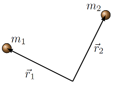
Fig. 2.13 Position vectors for two objects

Suppose you have two objects, each at some arbitrary location. We would denote the position vector of each object \(i = 1, 2\) as \({\vec r}_i\); to make it definite, let’s say they are masses \(m_i\), as in the picture above. The vector \({\vec r}_i\) will be a vector giving the location of the object \(i\) as seen from the origin of the coordinate system. In other words, \({\vec r}_i\) is a vector whose tail is at \((0, 0, 0)\), and whose tip is at the object \(i\). However, we often don’t care about where each object is, relative to the origin – the origin is a mathematical device we use to make the calculations easier. There is no special point in the Universe called “the origin”! Instead, we will care more about the relative position vector \({\vec r}_{ij}\), which is defined as

\[ {\vec r}_{ij} = {\vec r}_i - {\vec r}_j \]

This is the vector pointing from object \(j\) to object \(i\). In particular, \({\vec r}_{12}\) is a vector with its tail at \(m_2\) and its tip at \(m_1\); on the other hand, \({\vec r}_{21}\) is a vector with its tail at \(m_1\) and its tip at \(m_2\). The vector \({\vec r}_{12}\) is shown in the picture below. Notice that \({\vec r}_1 = {\vec r}_{12} + {\vec r}_2\) in terms of graphical vector addition!

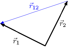
Fig. 2.14 Relative position vector for two objects

The index order is important

The relative position vector points from the second index object to the first. So, reversing the order of the indices flips the direction of the vector by 180\(^\circ\). As vectors, \({\vec r}_{ij} = -{\vec r}_{ji}\).

These relative position vectors will be used a lot when we define forces. For example, imagine you have two masses attached to each other by a spring. The spring force on each of the masses due to the spring will depend on the relative position vector between the mass and the equilibrium point of the spring. The larger this relative position vector is, the larger the size of the spring force acting on the mass.

Problem

Suppose that object 1 is at position \((1.25 \textrm{ m}) {\hat x} + (-0.750 \textrm{ m}) {\hat y}\) and object 2 is located at \((0.650 \textrm{ m}) {\hat x} + (0.350 \textrm{ m}) {\hat y}\). Find the vectors \({\vec r}_{12}\) and \({\vec r}_{21}\) in unit vector notation.

Answers: \({\vec r}_{12} = (0.600 \textrm{ m}){\hat x} + (-1.10 \textrm{ m}) {\hat y}\); \({\vec r}_{21} = (-0.600 \textrm{ m}) {\hat x} + (1.10 \textrm{ m}) {\hat y}\).

Problem

Write a vPython function relPosition() that uses arrows to show two vectors, and the relative position vector derived from them. Specifically, the function should take two vPython vectors vec1 and vec2 as arguments, representing the vectors \({\vec r}_1\) and \({\vec r}_2\). Then, it should create two vPython arrows representing those vectors, with their tails at the origin, and their tips at the positions given by \({\vec r}_1\) and \({\vec r}_2\). It should compute the relative position vector \({\vec r}_{12}\). Show this as a vPython arrow as well using graphical vector addition. In other words, the tail of \({\vec r}_{12}\) should be at the tip of \({\vec r}_2\). This gives a good check of the program, since this placement naturally puts the tip of \({\vec r}_{12}\) at the tip of \({\vec r}_1\). Finally, return the components of \({\vec r}_{12}\) as a vPython vector. Again, remember the ordering of the indices in \({\vec r}_{12}\) is important!

Answer: Here is a possible solution.

def relPosition(vec1, vec2):

    # Create arrows to represent vectors
    
    arr1 = arrow(pos = vector(0, 0, 0), axis = vec1, color = color.green, \
                 shaftwidth = 0.1)
    arr2 = arrow(pos = vector(0, 0, 0), axis = vec2, color = color.cyan, \
                 shaftwidth = 0.1)
    
    # Calculate the relative position
    # vector, and show as arrow
    
    vec12 = vec1 - vec2
    arr12 = arrow(pos = arr2.axis, axis = vec12, color = color.red)
    
    # Return relative position vector
    
    return vec12

2.4.5. Vector equations

As we have seen in this lesson, vectors have many mathematical operations that are similar to those for scalars. Specifically, vectors can be added together. We will see many cases where this happens; one prominent case is the addition of forces to get the net (or total) force. For example, suppose three forces \({\vec F}_i\) act on an object, but the net force is zero. This would be a vector equation of the form

\[ {\vec F}_1 + {\vec F}_2 + {\vec F}_3 = {\vec 0} \]

The zero vector

To emphasize the fact that this is a vector equation, I have set it equal to the zero vector \({\vec 0}\). This is the vector with all zero components, i.e.

\[ {\vec 0} = 0 {\hat x} + 0 {\hat y} + 0 {\hat z} \]

This is different than the scalar 0! I am underlining this point because the vector equation above for the three forces is really three scalar equations – one each for the \(x, y\), and \(z\) directions. By using good notation, we can put a lot of information into not very many symbols! So, scalars can add up to zero, like \(2 + (-2) = 0\), but vectors add up to the zero vector.

As another, more compact, way of showing the vector equation above, we can use the summation symbol \(\sum\). Here, we would write

\[ \sum_i {\vec F}_i = {\vec 0} \]

The left-hand side just means add up all of the vector \({\vec F}_i\) indexed by the letter \(i\). Here, \(i = 1,2, 3\) for the given forces. So, we have written the vector equation above, with three force vectors, in a different way. This can be useful, especially when the number of things being added together gets large. You may even see infinite sums in math class!

As an example of a vector equation, suppose we have two known vectors \({\vec A}\) and \({\vec B}\), and we want to find a third vector \({\vec C}\) such that \({\vec A} + {\vec B} + {\vec C} = {\vec 0}\). Then, this means that along each coordinate axis, the components also add up to zero; this is the “three for one” deal we get for vector equations. The vectors are written in unit vector form as \({\vec A} = A_x {\hat x} + A_y {\hat y} + A_z {\hat z}\), and similarly for the other two. So, the vector equation becomes the component equations

\[ A_x + B_x + C_x = 0 \qquad A_y + B_y + C_y = 0 \qquad A_z + B_z + C_z = 0 \]

Components are not vectors

Remember that the three scalars \(A_x, A_y\), and \(A_z\) represent the vector \({\vec A}\) in unit vector notation. It is important to keep the difference in mind!

Thus, the three components of \({\vec C}\) are

\[ C_x = -A_x - B_x \qquad C_x = -A_y - B_y \qquad C_x = -A_z - B_z \]

Let’s try this with some actual vectors, taking \({\vec A} = 5 {\hat x} - 7 {\hat z}\) and \({\vec B} = -2 {\hat x} + 3 {\hat y}\). Then, including the zeros for the missing components, we have \({\vec C} = [-(5) - (-2)] {\hat x} + [-(0) - (3)] {\hat y} + [-(-7) - (0)] {\hat z} = -3 {\hat x} - 3 {\hat y} + 7 {\hat z}\).

Problem

Suppose you are given the two vectors \({\vec J} = 8 {\hat y} + 2 {\hat z}\) and \({\vec L} = 5 {\hat x} + 8 {\hat y} - 5 {\hat z}\), and the vector equation \({\vec J} + {\vec K} + {\vec L} = {\vec 0}\). What is the vector \({\vec K}\), in unit vector notation?

Answer: \({\vec K} = -5 {\hat x} - 16 {\hat y} + 3 {\hat z}\).

Problem

You are given the vector equation \({\vec A} + {\vec B} + {\vec C} = {\vec 0}\). Write a vPython function missingVec() that finds the third vector satisfying this equation, given the other two. Specifically, the arguments of missingVec() are two vPython vectors, vecA and vecB. The function should calculate the vector \({\vec C}\) and return its components.

The function should also show the graphical vector addition the vector equation represents. In other words, the function must create three vPython arrow objects, and arrange them tip-to-tail, to show that the three vectors add together to the zero vector. Hint: Remember that for an arrow object arrObj with position attribute arrObj.pos and axis attribute arrObj.axis, the tip of the arrow is located at the position vector arrObj.pos + arrObj.axis.

Answer: Here is an example of such a vPython function.

def missingVec(vecA, vecB):

    # Find third vector C such that
    # A + B + C = 0
    
    vecC = -(vecA + vecB)
    
    # Create arrow objects for each vector
    
    Aarr = arrow(pos = vector(0, 0, 0), axis = vecA, color = color.green, \
                 shaftwidth = 0.1)
    Barr = arrow(pos = Aarr.axis, axis = vecB, color = color.cyan, \
                 shaftwidth = 0.1)
    Carr = arrow(pos = Barr.pos + Barr.axis, axis = vecC, \
                 color = color.red, shaftwidth = 0.1)
    
    # Return vector C components

    return vecC

2.5. Summary

In this lesson, you have learned about vectors, one of the fundamental objects we will use throughout this course to describe both the motion of objects – such as position, velocity, and acceleration – and the properties that determine that motion – for example, momentum, forces, and fields. The technique of graphical addition, either drawing by hand or using vPython to create the arrows can demonstrate the appearance of the scalar multiple of a vector, or of a vector sum. These methods will be put in practice often (starting with the next lesson!), so you should make sure you have a firm grasp of these topics.

After this lesson, you should be able to

• Using graphical vector methods, add or subtract vectors

• Given the components of a vector,

  • write the vector in proper unit vector notation

  • multiply the vector by a scalar

• Given the components of two or more vectors, find the vector sum of the vectors

• Create an arrow in vPython

• Show the vector sum of two or more vectors using vPython arrows

1. Introduction to Python 3. Velocity and the Euler method