25. Electric fields¶

25.1. Overview¶

Links to programs in this lesson:

Find the net electric field
Motion in a constant gravitational field

The physicist of today is well versed in the use of Newton’s second law and forces acting on an object. However, these methods are restricted to physical objects (balls rolling down ramps), and do not map over to other situations. In fact, it is much easier to deal with electricity and magnetism when using a more general idea, known as a field. It was this conceptual leap in the mid-19th century that eventually set the stage for the quantum mechanical revolution of the early 20th century. Thus, the fundamental theories of physics are written as quantum field theories (and not “force theories”!).

The concept of a field was developed by two great scientists – the experimentalist Michael Faraday, and the theoretical physicist James Clerk Maxwell. Faraday, a self-taught physicist, was the first to lay out a vision of electric and magnetic phenomena arising from ‘’lines of force’’ – physical tubes forming space and affecting the motion of charged particles moving through space. This was more of a philosophical viewpoint on experimental results, rather than a systematic picture. Then, Maxwell developed a more mathematical framework, writing down what are now known as Maxwell’s equations for the electric and magnetic fields. These equations were the inspiration for much of modern physics, including Einstein’s theory of special relativity, and the quantum field theories used to explain interactions at the subatomic scale.

We have already seen the gravitational field, as a different way of describing the influence of gravity on the motion of an object. In this lesson, we do the same thing for charged objects, developing the electric field from the electrostatic force.

Since electric fields are something that many do not have a good intuitive feel for, it may be helpful here to remember what the idea of a field is. I like to do this with the following analogy. Suppose you need to buy some bread, in order to make sandwiches. You go to the store, and see that loaves of bread are on sale for $2 per loaf. This will be the price that everyone agrees on (no haggling allowed!). So how many loaves are you buying? If you are making sandwiches just for yourself, one loaf will probably last you the week; you will have to spend $2. However, if you need to feed the entire battalion, you may need to buy 100 loaves, and use $200 to do so. The price you pay for the bread is different if you get different amounts, but the price per loaf always stays the same! This is the idea behind a field. Everyone agrees on the size of the gravitational field (force per kilogram – same as the price per loaf), but different objects have different forces (total price), since they have different masses. We will see the same idea carries over to electric fields, which will be force per charge, instead of per mass.

Here are the objectives for this lesson:

State the definition of the electric field in terms of the electrostatic force on a test charge, and identify its units.
Describe the relationship between the direction of the electric field and the direction of the electric force on a point charge.
State the equation for the electric field created by a point charge.

25.2. Electric fields¶

Throughout this lesson, we will use the gravitational field ${\vec g}$ as a stepping stone to understanding the electric field ${\vec E}$. It may help to go back to gravitational fields in Lesson 21 where we talked about ${\vec g}$ in some detail. Remember that the gravitational field is defined as

\[ {\vec g} = \frac{{\vec F}_g}{m} \]

where $m$ is the test mass used to measure the gravitational field at its location. The gravitational field at this location gives a measure of the influence at that point of all the surrounding masses. The idea is to “factor out” the size of the test mass, so that we are only measuring the gravitational effects of all these other masses around the test mass’ location. Note that the gravitational force ${\vec F}_g$ and the gravitational field ${\vec g}$ always point in the same direction, since the mass $m > 0$ for all objects.

We can now define the electric field in the same way, by analogy – using a test charge $q$ instead of mass $m$, and electrostatic force ${\vec F}_e$ instead of gravitational force ${\vec F}_g$.

Quantity: electric field
Symbol: ${\vec E}$
Definition: The electric field at a given location is found by dividing the electrostatic force on a test charge at that location by the test charge.

\[ {\vec E} = \frac{{\vec F}_e}{q} \]

SI units: newtons per coloumb (or N/C)

It helps to think conceptually about what we are doing: we want to find a quantity ${\vec E}$ that gives the influence of a collection of charges at a particular point $P$, so we place a test charge $q$ at this point $P$. However, we want our answer ${\vec E}$ not to depend on what test charge we use, so we “factor out” the size of the charge $q$ from the electrostatic force. Thus, if you use a large, positive test charge, and I use a small, negative test charge, the electrostatic forces on our charges will be different, but the electric field ${\vec E}$ we measure will be exactly the same!

Let’s talk about the direction of the electric field first. We can use the definition of the electric field to find the direction of the electric field, due to a single charge $Q$. In particular, suppose there is a charge $Q > 0$ creating an electric field we want to measure. You use your positive test charge $q_+$ to find the electrostatic force on your charge, as seen in the picture below. Since both charges are positive, the test charge is repelled from the charge $Q$. Then you divide the electrostatic force $F_e$ on $q_+$ by the charge $q_+$ (using the definition of electric field above) to get the electric field at the point you placed the test charge. Because $q_+ > 0$, the electrstatic force ${\vec F}_e$ and the electric field ${\vec E}$ point in the same direction – away from $Q$.

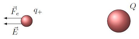
../_images/INT_AY21_L29_Fig03_Pos_test_charge.png

Fig. 25.1 Using a positive test charge $q_+$ to measure the electric field due to charge $Q$¶

After you do that, I decide to check your answer by using my negative test charge $q_-$. Again, I find the electrostatic force on $q_-$ due to $Q$, and then divide out by $q_-$ to get ${\vec E}$. Since $q_- < 0$, the two charges now attract, but dividing the force vector by a negative number gives an electric field that points in the opposite direction. But this is the same direction that you found with your positive test charge! Everyone agrees on the size and direction of the electric field, regardless of what test charge they use to measure it.

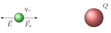
../_images/INT_AY21_L29_Fig04_Neg_test_charge.png

Fig. 25.2 Using a negative test charge $q_-$ to measure the electric field due to charge $Q$¶

Following this logic, we can now find the direction of the electric field due to a single charge $Q$:

The electric field created by a positive charge points away from that charge.
The electric field created by a negative charge points towards from that charge.

Rule of thumb for electric field direction

Since the electric field always points in the same direction as the electrostatic force on a positive test charge, you can just ask yourself which way the force is on a positive test charge placed at the point of interest, in order to get the direction of the electric field at that point.

If you use the PhET below, you can play around with the electric fields due to collections of positive and negative charges. The PhET app will show you the total electric field vectors at a grid of points. This ${\vec E}_{net}$ is the vector sum of all the individual electric fields, so its direction can change depending on the size and sign of the individual charges creating the net field.

25.3. Electric fields of point charges¶

Now let’s talk about an important special case. The definition given above for the electric field works for any situation, such as an extended charge (such as a charged disk or rod). Frequently, however, we will only need to find the electric field due to one or more point charges $Q$. Thus, we can start with Coulomb’s law for the electrostatic force between two charges. We will find the field a distance $d$ away from charge $Q$ by placing a test charge $q$ there, at a point I will call $P$, and find the electrostatic force on it. I use $d$ instead of $r$ for the distance, so we do not confuse it with the unit vector ${\hat r}_{PQ}$. The situation is shown in the diagram below.

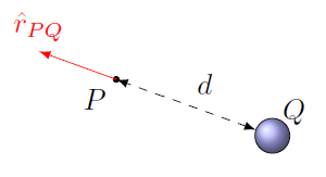
../_images/INT_AY21_L29_Fig09_Field_at_point.png

Fig. 25.3 Finding the electric field ${\vec E}_P$ at point $P$, due to a charge $Q$¶

From Coulomb’s law, this would be

\[ {\vec F}_e = \biggl( \frac{kqQ}{d^2} \biggr) {\hat r}_{PQ} \]

Here, the unit vector ${\hat r}_{PQ}$ is at the point $P$, and points away from the charge $Q$. Thus, if we now use the definition of electric field we find that dividing by $q$ gives

\[ {\vec E} = \biggl( \frac{kQ}{d^2} \biggr) {\hat r}_{PQ} \]

Notice what happens here – since ${\hat r}_{PQ}$ points away from the charge $Q$, if that charge is positive, then the electric field at point $P$ due to charge $Q$ also points away from $Q$. On the other hand, if $Q$ is a negative charge, the electric field points towards $Q$. This matches what I said earlier about the directions, so everything works out!

Problem

Two identical positive charges are shown in the figure below. Which direction is the electric field at point $P$ due to these two charges? Choose the appropriate number for the direction, or ‘0’ if the field is zero.

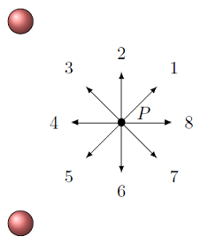
../_images/INT_AY21_L29_Fig05_Field_from_two_pos_charges_small.png

Fig. 25.4 Electric field from two identical positive charges¶

Answer: The electric fields due to the individual positive charges are both away from the charge. Thus, the vector sum of the fields is to the right, or choice 8.

Problem

A positive charge (at top) and a negative charge (at bottom) of identical size are shown below. Which direction is the electric field at point $P$ due to these two charges? Choose the appropriate number for the direction, or ‘0’ if the field is zero.

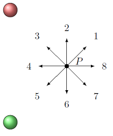
../_images/INT_AY21_L29_Fig06_Field_from_dipole_small.png

Fig. 25.5 Electric field from positive and negative charges¶

Answer: The electric field due to the positive charge is away from it, while the electric field due to the negative charge is towards it. The vector sum of these fields is towards the bottom of the page/screen, or choice 6.

Problem

Two identical positive charges are shown in the figure below. Which direction is the electric field at point $P$ due to these two charges? Choose the appropriate number for the direction, or ‘0’ if the field is zero.

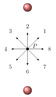
../_images/INT_AY21_L29_Fig07_Field_from_two_pos_charges_small.png

Fig. 25.6 Electric field in between two identical positive charges¶

Answer: Since the two charges are both equal in size and positive, and the same distance from the point, their electric fields are equal in magnitude, but opposite directions (away from each charge). Thus, the two fields cancel out, and the net electric field is zero.

We now have an equation for the electric field at some point $P$ a distance $d$ away from a charge $Q$. We use this in an example in the next section.

25.4. Example: Equilateral triangle, again¶

Let’s see how the electric field captures the influence of charges, for any test charge used, by returning to the example from Lesson 24 (Coulomb’s law) with charges on the corners of an equilateral triangle. Much of the notation we use below will be the same as that example, so it may be helpful to go back to it and review it.

For now, let’s only put two charges on the triangle, and leave the third corner empty. We will now find the electric field at this empty corner $C$. Remember that the two charges were $q_2 = -4.00 \ \mu C, q_3 = +3.00 \ \mu C$, and the side lengths were $d = 7.00$ m.

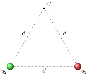
../_images/INT_AY21_L29_Fig08_Field_at_triangle_corner_small.png

Fig. 25.7 Find the electric field at point $C$ due to the two charges $q_2, q_3$¶

We now find the electric field ${\vec E}_2$ at point $C$ due to charge $q_2$, and similiarly ${\vec E}_3$ at $C$ due to $q_3$. Based on the directions we talked about in the last section, ${\vec E}_2$ will point towards $q_2$, since it is a negative charge, while ${\vec E}_3$ will point away from $q_3$. To flesh this out, remember that the unit vectors at point $C$ are given by

\[ {\hat r}_{C2} = (\cos \theta) {\hat x} + (\sin \theta) {\hat y} \qquad {\hat r}_{C3} = (-\cos \theta) {\hat x} + (\sin \theta) {\hat y} \]

We can use these to find the electric fields. Much like we drew a FBD for forces, we will do something similiar with electric fields, by drawing an electric field diagram (or EFD) to show all of the individual electric field vectors at a particular point. For this situation, at point $C$, the EFD would look like the picture below, since the field ${\vec E}_2$ points towards the negative charge $q_2$, while the field ${\vec E}_3$ points away from the positive charge $q_3$.

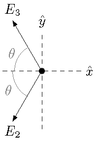
Fig. 25.8 Electric field diagram at the point $C$¶

The electric field ${\vec E}_2$ at point $C$, due to charge $q_2$, is then

\[ {\vec E}_2 = \biggl( \frac{kq_2}{d^2} \biggr) [(\cos \theta) {\hat x} + (\sin \theta) {\hat y}] \]

and the electric field ${\vec E}_3$ because of charge $q_3$ is

\[ {\vec E}_3 = \biggl( \frac{kq_3}{d^2} \biggr) [(-\cos \theta) {\hat x} + (\sin \theta) {\hat y}] \]

Plugging in the numbers (with $\theta = 60.0^\circ$) gives

\[ {\vec E}_2 = (-366.9 \textrm{ N/C}) {\hat x} + (-635.6 \textrm{ N/C}) {\hat y} \]

and

\[ {\vec E}_3 = (-275.2 \textrm{ N/C}) {\hat x} + (476.7 \textrm{ N/C}) {\hat y} \]

As expected, these vectors match those we put into the EFD above. Thus, the total electric field at point $C$ due to the two charges at the other corners is

\[ {\vec E}_{net} = (-642.1 \textrm{ N/C}) {\hat x} + (-158.9 \textrm{ N/C}) {\hat y} \]

Now, let’s talk about the benefit of using the electric field. This field ${\vec E}_{net}$ is the same, regardless of what charge is placed there. This provides a quick way of finding the electrostatic force acting on a charge $q_1$ placed at the corner $C$. To show this, we can quickly compute the force on the charge $q_1 = +2.00 \ \mu C$ we used in the Lesson 24 example. Then, from the definition of electric field, the net force ${\vec F}_1$ on charge $q_1$ is just

\[ {\vec F}_1 = q_1 {\vec E}_{net} \]

and you can quickly verify that this gives the same answer we found in Lesson 24.

Forces and fields

If you know one of either the electric field at a point, or the electrostatic force on a charge at the same point, and are asked to find the other, don’t solve from scratch! It is much easier to use the definition of the electric field to simplify the calculation.

To emphasize the point, as one example we can see that the electric field due to charge $q_2$ is “inside” the electrostatic force between charges $q_1$ and $q_2$ by

\[ {\vec F}_{12} = \biggl(\frac{k q_1 q_2}{d^2} \biggr) [(\cos \theta) {\hat x} + (\sin \theta)] = q_1 {\vec E}_2 \]

Because of the form of Coulomb’s law, the charge at the point in question will always factor out like this, and the remainder of the equation will be exactly the electric field due to the other point charge.

As we did in the last lesson, we can write a vPython function that finds the electric field at a point, due to a list of other charges. Because we “divide out” by the test charge, then we only need the location to find the field, and the charges creating the field. This is done by the function netElecField() in the Trinket app below.

Back to program list

Let’s briefly talk about the heart of the function netElecField(); this is very similar to what we did with the function netElectroForce() in Lesson 24. The important command in the function here is

netField += (k * otherObj.charge / r ** 2) * rHat

This matches with the physics equation

\[ {\vec E}_{Pj} = \biggl( \frac{k q_j}{r^2 _{Pj}} \biggr) {\hat r}_{Pj} \]

As in Lesson 24, the point charge $q_j$ is given in vPython as otherObj.charge. The vPython vector rVec gives the relative position of the point $P$ as seen by the charge $q_j$, i.e. the vector ${\vec r}_{Pj}$. Finding the unit vector in the same direction as ${\vec r}_{Pj}$, by using hat(rVec), gives the vector ${\hat r}_{Pj}$. The magnitude $r$ of ${\vec r}_{Pj}$ is found with the command mag(rVec). Just like the electrostatic force, everything in the parentheses is a scalar, so the fact that netField is a vector comes solely from the unit vector rHat.

Problem

Three charged particles are located on the corners of a rectangle, as shown below, with $x = 7.50$ cm and $y = 5.00$ cm. The charges are $q_1 = +3.30 \ \mu$C, $q_2 = -7.89 \ \mu$C, and $q_3 = +4.25 \ \mu$C. Find the net electric field at the fourth corner, marked by the point $P$. Give the magnitude in MN/C, and the direction in degrees CCW from the $+x$ axis.

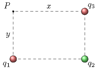
../_images/INT_AY22_L29-Fig01_Charges_on_rect.png

Fig. 25.9 Find the net electric field at the marked point $P$¶

Answer: ${\vec E}_P = 7.04$ MN/C at 86.2$^\circ$ CCW from the $+x$ axis

Problem

Use the program above, and the function netElecField(), to check your answer for the previous question.

Answer: To carry this out, you need to change the commands after the definition of the function netElecField() to read the following. This will give the vector in unit vector form, which you can find the magnitude and direction of, either by direction calculation, or else using a vPython program similar to that given at the end of Lesson 24.

# Definitions

x = 0.0750               # Horiz. rectangle side (m)
y = 0.0500               # Vert. rectangle side (m)

# Create point P, charges

point = sphere(pos = vector(0, y, 0), color = color.white, \
               radius = 5E-3)
q1 = sphere(pos = vector(0, 0, 0), charge = 3.30E-6, \
            color = color.red, radius = 5E-3)
q2 = sphere(pos = vector(x, 0, 0), charge = -7.89E-6, \
            color = color.green, radius = 5E-3)
q3 = sphere(pos = vector(x, y, 0), charge = 4.25E-6, \
            color = color.red, radius = 5E-3)

# Find net electric field at P, due to charges

result = netElecField(point.pos, [q1, q2, q3])
print('Net electrostatic field at P =', result, ' N/C')

25.5. Field lines¶

25.5.1. Gravitational field lines¶

A very helpful way of showing the strength and direction of the electric field in a region of space is by drawing the field lines. These are a pictorial representation of the electric field, much like a contour map shows the altitude of a surface. Using electric field lines is helpful is gauging both the direction of the field, as well as the relative strength of the field, at various locations. To start, it may be helpful to think of this first in terms of the gravitational field, something we are more familiar with, so I will use this as an example to build up to electric field lines.

As we all learned in the cradle, the gravitational field near the surface of the Earth is 9.81 m/s$^2$ pointing downward (there are actually small variations, but we will ignore those). What this means is that if I throw a test mass into the air anywhere on the Earth’s surface, then ignoring air resistance, the acceleration of that mass will be downward. If I have a bunch of such test masses, and I draw arrows showing the gravitational field at each of them, it would look like the picture below.

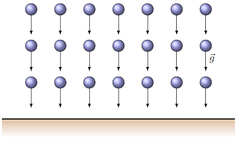
../_images/INT_AY21_L29_Fig01_Grav_field_vectors_small.png

Fig. 25.10 Gravitational field vectors for a group of test masses near the surface of the Earth¶

It starts being messy to draw both the objects and the fields, so what we do is connect the field vectors to give lines, in such a way that at every point on the line, the gravitational field vector is tangent to the line. This acts like a “contour map” of the gravitational field near the ground. Taking the picture above, this would give the gravitational field lines shown below.

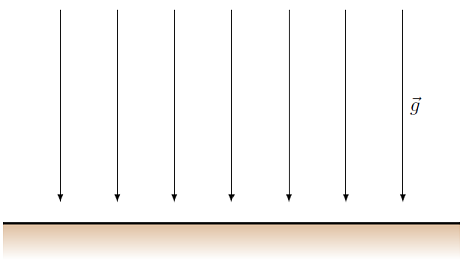
../_images/INT_AY21_L29_Fig02_Grav_field_lines_small.png

Fig. 25.11 Gravitational field lines near the surface of the Earth¶

Already, we can easily see the direction of the gravitational field, pointing downward towards the surface. In addition, the fact that the field lines are the same distance apart actually tells us that the gravitational field has a constant magnitude in this representation. We will talk more about this further on.

Field lines are not trajectories

It is important to note that the field lines shown above do not represent the motion of a mass in the gravitational field. Instead, they give the direction of the gravitational field, which in turn tells you about the acceleration of the object. You can see that by running the program below. The cyan arrows represent the constant gravitational field lines near the ground. On the ball itself, the magenta arrow shows the ball’s velocity, and the white arrow its acceleration. The white arrow will always match the field at that location, but the trajectory of the ball is not straight down because of its non-zero $v_x$ component.

The Trinket app below shows the relation between the gravitational field lines, and the motion of a projectile. We have seen this case in Lesson 04, when we considered projectile motion. Near the surface of the Earth, the gravitational field is constant, which tells us the acceleration of a ball, but not the velocity. Thus, if you run the simulation below, you will see that the ball does not move directly along the gravitational field vectors, but instead those vectors give the direction of the ball’s acceleration.

Back to program list

25.5.2. Electric field lines¶

Now we turn to drawing the electric field lines due to various charges. The logic is the same as for the gravitational field lines given above – we imagine placing test charges at many locations in space, and uses the electric field vectors at each of these locations to map out the continuous electric field lines. If we do this around a single positive charge, and then a single negative charge, the resulting electric field lines look like the two figures below.

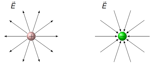
../_images/INT_AY20_MP3_L03_Fig01-Electric_field_lines_of_pt_charges_small.png

Fig. 25.12 Electric field lines around single point charges¶

First, the direction of the field lines is the same as what we said earlier: towards a negative charge, and away from a positive charge. In addition, the field lines get further apart as you move away from each charge. Remember that the electric field is an inverse square law, so that the magnitude $E \sim 1/r^2$. Thus, the fact that the field lines spread apart is a visual indication that the electric field magnitude is getting smaller with increasing distance $r$. Finally, since the electric field measured by a test charge placed at a particular point can only point in a single direction, that will be the direction of the electric field line going through the same point. In other words, electric field lines cannot cross, since this uniqueness would be violated.

Properties of electric field lines

Electric field lines start at negative charges and end at positive charges.
The electric field is stronger when the electric field lines are closer together, and weaker when they are farther apart.
Electric field lines never cross.

The next two problems show how you can use the electric field lines around point charges in order to ascertain properties of these charges.

Problem

What are the signs of the charges whose electric fields are shown below?

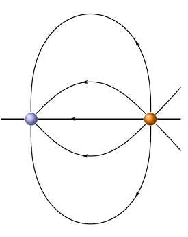
../_images/INT_AY20_MP3_L03_Fig02-E-field-lines-of-two-charges_small.png

Fig. 25.13 Electric field lines of two charges¶

Answer: The blue charge is negative, the orange charge is positive.

Problem

Using the same picture as the previous problem, which of the two charges has the greater magnitude?

Answer: If you count the number of electric field lines incident on each charge, there are two more touching the orange charge than the blue. Thus, the density of field lines is greater around the orange charge, implying it has the greater size of charge.

The final problem uses many of the ideas of this lesson – namely the definition of the electric field itself, and of electric field lines.

Problem

A $+4.00$ C charge is placed in a uniform electric field, and it feels an electrostatic force of magnitude 12.0 N. If this charge is removed and a $+6.00$ C charge is placed at the same point, what force will it feel?

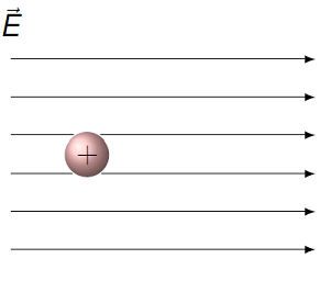
../_images/INT_AY20_MP3_L03_Fig03-Charge-in-uniform-E-field_small.png

Fig. 25.14 Charge placed in a uniform electric field¶

Answer: 18.0 N/C, to the right

25.6. Summary¶

As stated in the introduction of this lesson, the concept of fields is the basis of much of modern physics. We had previously seen the gravitational field. The “9.81 m/s$^2$” you have memorized is just the magnitude of the Earth’s gravitational field near its surface; however, such fields are present everywhere in the Universe. Now we have a similar idea for the electric field. Because most things do not have a net charge, electric fields are not as ubiquitous as the gravitational variety. However, for a great range of technological devices, it is important to know something about these fields. For example, in some applications, you want to shield your electronics from too large of a field, to avoid failure; in other places, you are interested in creating as large a field as possible, to increase the signal strength for your communications or detection devices.

Yet we are really only talking about one aspect of the combination “electromagnetism”, where both electric and magnetic fields are used together. We have already seen electric fields, and built up some intuition about them, starting from our everyday experience with the gravitational field. We will now complete this picture by introducing magnetic fields in the next lesson.

After this lesson, you should be able to:

State the direction of the electric field due to a point charge.
Calculate the electric field at a specified point due to a collection of charges.
Interpret the electric field lines of a given situation.

NAPS Intermediate Physics

25. Electric fields¶

25.1. Overview¶

25.2. Electric fields¶

25.3. Electric fields of point charges¶

25.4. Example: Equilateral triangle, again¶

25.5. Field lines¶

25.5.1. Gravitational field lines¶

25.5.2. Electric field lines¶

25.6. Summary¶