27. Biot-Savart law
Links to programs in this lesson:
What we now call “electricity” and “magnetism” have been familiar to many for over two thousand years. However, for much of that time, they were interesting effects, and not much else; there was no theory behind the existence of electric and magnetic properties. In fact, although some had suspected a relationship between them, nothing definite was known. This began to change in the 18th and 19th centuries, as technology advanced to the point where they could be studied. In particular, with the development of the electric battery by Volta in 1800, a continuous electric current was possible.
A bridge between electricity and magnetism was first built by the efforts of the Danish physicist and chemist Hans Christian Oersted, who did the necessary experiments around 1820. In these, he showed that a constant electric current through a wire produced a magnetic field. Again, it is useful to take a moment and think how important this result was. Although electric and magnetic fields have some similarities (as discussed in Lesson 34), this does not necessarily mean they are one and the same phenomenon. However, it was the results of Oersted, and many others in the next few years, who conclusively showed that we should not think of “electricity” and “magnetism” separately, but instead to put it into “electromagnetism”.
Although we will not get into this further in this course, the unification of electricity and magnetism was an important event in the history of physics. Over the next 175 years or so, the main course of theoretical physics was a similar path of unification, using many mathematical ideas first developed for electromagnetism. The fruits of this are in what is known as the Standard Model of particle physics, joining electromagnetism together with the strong nuclear force (keeping nuclei together) and the weak nuclear force (responsible for radioactive decay). The Standard Model uses the idea of fields as a basic component, and represents our best current knowledge of how fundamental physics works.
In this lesson, we will answer a basic question: where do magnetic fields come from? Shortly after Oersted published his experiments, a key part of the answer was found by two physicists, Jean-Baptiste Biot and Felix Savart, building off the idea of the motion of electric charge in a current giving a magnetic field. We will explore their results in this lesson.
27.1. Overview
Here are the objectives for this lesson:
State the Biot-Savart law
Find the magnetic field at a given distance away from a long, straight wire.
Calculate the magnetic field due to a current of a given shape.
27.2. Long, straight wires
Before we state the Biot-Savart law, let’s first talk about what Oersted found in his experiments. Suppose we have a long, straight wire; basically, we are considering a straight wire whose length is much greater than its radius (or thickness). Oersted sent a current through such a wire, and saw that a nearby compass changed its direction every time he did this. When he turned off the current, the compass returned to its original orientation. Oersted grasped that this was because the current in the wire was creating a magnetic field of its own! After some confusion about the direction of this field, Oersted finally realized that the magnetic field around the wire is circular. In other words, we would say that the magnetic field lines are circles, with their center at the wire itself. You can see a reproduction of Oersted’s experiment in the video given below (source). When there is no current through the wire, the compass points in the direction of the Earth’s magnetic field. However, when the voltage source is turned on, and current flows through the wire, the compass shifts to point in the direction of the much stronger magnetic field of the wire.
In order to see the magnetic field more clearly, you can run the vPython program below. This shows the magnetic field vectors at various points around a long, straight wire. These vectors form circles, with the wire at its center.
Notice the relationship between the direction of the current \(I\) through the wire, and the circular magnetic field lines around the wire. This is given by a version of the right-hand rule. Imagine that you are grabbing the wire with your right hand. When you point the thumb of your right hand in the direction of the wire’s current, your fingers will naturally curl in the direction of the magnetic field lines. For example, if you see the current moving upward, then with your right thumb pointing upward as well, your fingers will go right to left behind the wire, and left to right in front of the wire. We will see later in this lesson how to relate this to the right-hand rule we saw in Lesson 34 for the magnetic force.
Problem
A positive charge moves parallel to a wire. If a current is suddenly turned on, in which direction will the magnetic force act on the charge?
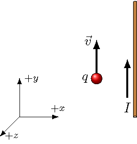
Fig. 27.1 Positive charge moving along a current-carrying wire
\(+z\) (out of page)
\(-z\) (into page)
\(+x\)
\(-x\)
\(-y\)
Answer: You can use the right-hand rule described above to find the direction of the magnetic field due to the wire. At the location of the positive charge \(q\), this field \({\vec B}\) points in the \(+z\) direction. Then, using either the vector product, or the right-hand rule, to find the direction of the magnetic force \({\vec F}_{mag}\), this gives the force points in the \(+x\) direction, or toward the wire.
Soon after Oersted announced his discovery, the French scientist Andre-Marie Ampere (whom the unit of current was named after) studied the effects of current-carrying wires on each other. Because each wire produces its own magnetic field, the field due to one wire will create a force on the other. This leads to the wires attracting or repelling each other, depending on the current through each.
Let’s see how this works, by first seeing how a magnetic field affects a wire with a current passing through it. This will built on the previous problem. From the last lesson, we have that the magnetic force \({\vec F}_{mag}\) on a single charge \(q\), resulting from placing the charge in a magnetic field \({\vec B}\), is given by
Now, a current \(I\) is simply a collection of charges \(\Delta Q\) moving past a given point within a time interval \(\Delta t\), with \(I = \Delta Q / \Delta t\). Suppose the charges are moving down a wire with a displacement \({\vec \ell}\); I am using a little different notation here, to avoid confusing symbols when we get to the Biot-Savart law. With a velocity \({\vec v} = {\vec \ell} / \Delta t\), then we have that
Thus, for a collection of charges \(\Delta q\), we can replace \((\Delta q) {\vec v}\) in the magnetic force equation with \(I {\vec \ell}\), resulting in the magnetic force on a current-carrying wire as
Again, \(I\) is the current through the wire, whose length and direction are given by the vector \({\vec \ell}\).
Notice that the force on the wire points in the same direction as the force on the individual charges. Hopefully this is a sensible result! But it also allows us to predict the results of Ampere’s experiments on the forces between wires. For now, we will only find the direction of this force. After we talk about the Biot-Savart law, we will return to this force, and calculate the magnitude as well.
Problem
Two straight wires run parallel to each other, carrying currents in the directions shown. The two wires experience a force in which direction?
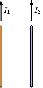
Fig. 27.2 Two parallel current-carrying wires
away from each other
towards each other
there is no force
Answer: Remember that current is conventional current, i.e. considered as the flow of positive charges. Thus, you can use the same steps as the previous problem to find the force on the left-hand wire due to the magnetic field from the right-hand wire. The left-hand wire will be attracted to the right-hand wire.
We can do the same thing for the right-hand wire, thinking of the current as the flow of positive charges towards the top of the page/screen. At this wire, the magnetic field due to the left-hand wire will be into the page/screen. Using the right-hand rule gives that the force on this current is to the left.
Thus, the two wires will be attracted to each other, due to the magnetic forces on each from the magnetic field of the other wire.
27.3. The Biot-Savart law
As we saw, Oersted found that the magnetic field lines around a long, straight wire are circles centered on the wire. So how can we extend this to more complicated wires? We will follow a similar path to what we have done with previous fields: build up the complicated cases as a sum of a lot of simple cases. In particular, imagine that we have a small bit of wire; this is represented by the vector \(\Delta {\vec \ell}\), where \(\Delta \ell\) is a small length. Flowing through this wire is a current \(I\). The direction of the vector \(\Delta {\vec \ell}\) gives the direction of this (conventional) current.
Now, imagine that we want to find the magnetic field vector at a point \(P\). To do this, we need the position vector of \(P\) relative to the wire. This is given by \({\vec r}\) – this vector starts at the center of the wire \(\Delta {\vec \ell}\), and points towards the point \(P\). To see this set-up, run the program below. The green cylinder is the wire, with the current shown by the white arrow inside of it. The position vector \({\vec r}\) is the yellow arrow from the wire to the point \(P\) to the left of the screen.
Now, according to Biot and Savart, the current in the wire will then produce a magnetic field \(\Delta {\vec B}\) at the point \(P\), given by
There is a lot we have seen before here, but let’s break it down, since it is put together differently than the corresponding equations for the gravitational and electric fields. As Oersted saw, the magnetic field size depends on the value of the current, so it is appropriate it appears in the numerator. In the denominator, we also see the usual \(r^2\) distance dependence we would expect from an inverse-square law. Finally, we also have a new physical constant, the vacuum permeability \(\mu_0\), given by
This constant gives the relationship between the sources of a magnetic field, and the size of the field created by that field. A fun fact: this constant used to be defined as exactly \(4\pi \times 10^{-7}\) N/m, but after the SI unit system was redefined in 2019, this is no longer true. However, it is awfully close, so I will often pretend that this definition still holds.
Problem
If I use \(\mu_0 = 4\pi \times 10^{-7}\) N/m, what is the error, compared to the actual defined value \(\mu_0\) given above?
Answer: The error is given by \(\mu_0/(4\pi \times 10^{-7}) - 1 = 5.44 \times 10^{-10}\). Good enough!
Oersted also saw that the magnetic field lines were circles – how do we get that from the vector product above? Well, remember that the vector product \({\vec A} \times {\vec B}\) is always perpendicular to the plane defined by the vectors \({\vec A}\) and \({\vec B}\). This is what we get here. In the program above, the vector \(\Delta {\vec \ell}\) along the wire points in the \(+y\) direction. The position vector \({\vec r}\), from the wire to the point \(P\), is in the \(-x\) direction, which means that the unit vector \({\hat r}\) points in the same direction. So, using the right-hand rule with the vector product \(\Delta {\vec \ell} \times {\hat r}\) give that it points in the \(+z\) axis. Notice that this is exactly what I said earlier with the “right-hand rule” using currents and the circular magnetic fields! Point your thumb in the direction of the current (\(+y\)), and your fingers will naturally point towards you on the left side of the wire.
27.4. Magnetic field at center of a circular wire
Let’s now go through our first example of using the Biot-Savart law: finding the magnetic field at the center of a circular wire with a current through it. You might be surprised that we are not finding the field at some point near a long, straight wire, but it turns out the circular loop of wire is actually an easier place to start! Imagine we have a circular loop with a radius \(R\) and a current \(I\) flowing through it. We want to find the total magnetic field \({\vec B}\) at the point \(P\), at the center of the circular wire. To do this, we can pretend that the circle is a regular polygon with a large number of sides \(N\), and add up the contributions from the current flowing through each of these sides. Then, making \(N\) larger and larger will get us closer to the final answer.
The picture below shows the basic set-up for approximating the circle by a polygon. The green sides represent the polygon (here with \(N = 12\) sides), while the dotted line is the circle the polygon is used to estimate. We will need to find algebraic expressions for the vectors \({\vec r}\) and \(\Delta {\vec \ell}\), for a given angle \(\theta\), in order to find the magnetic field at the center point \(C\).
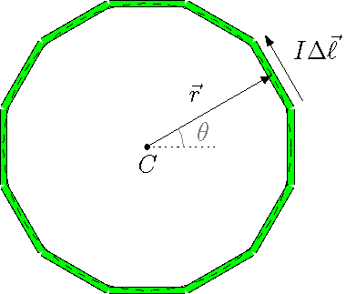
Fig. 27.3 Polygonal approxmation for a circle
Now, I have used the “usual” way of defining the position vector \({\vec r}\), namely from the point \(C\) to the center of the wire segment \(\Delta \ell\). But this is actually backwards from how \({\vec r}\) is defined in the Biot-Savart law! Remember that, in that equation, \({\vec r}\) points from the wire segment to the observation point. Since we are more used to working with \({\vec r}\) starting at the origin, I will keep it that way for now, just remember that I will really need \(-{\vec r}\) when I put everything back into the Biot-Savart law.
Let’s now find the vectors \({\vec r}\) and \(\Delta {\vec \ell}\); for each side of our polygon, the length vector \(\Delta {\vec \ell}\) is perpendicular to the radius vector \({\vec r}\) to the center of that side. Thus, if \({\vec r} = (R \cos \theta) {\hat x} + (R \sin \theta) {\hat y}\), then \(\Delta {\vec \ell} = [-(\Delta \ell) \sin \theta] {\hat x} + [(\Delta \ell) \cos \theta] {\hat y}\). Notice that I have chosen the direction of \(\Delta {\vec \ell}\) so that the current (with \(I > 0\)) flows in the counterclockwise direction, when we look down from the \(+z\) axis.
Problem
Use the scalar product to show that the vectors \({\vec r}\) and \(\Delta {\vec \ell}\) just given are perpendicular for all angles \(\theta\).
I want to flesh out the process for finding the vectors \(\Delta {\vec \ell}\) – where do these vectors come from? Remember we want to approximate the circle as a polygon, so we can choose points on the circle as the “corners” of the polygon. Then, each side has a vector \(\Delta {\vec \ell}\) starting at the point \(P_k\), and ending at the next counterclockwise point \(P_{k + 1}\). How do we find these points? Since we are dividing the circle into \(N\) parts, each point \(P_k\) is an angle \(2\pi k/N\) along the circle from the \(+x\) axis. This is because we take the total angle \(2 \pi\) (in radians), and divide it into \(N\) pieces. Thus, point \(P_k\) has a position vector
Therefore, the vector along the side from point \(P_k\) to point \(P_{k + 1}\) is simply the vector difference \({\vec r}_{k + 1} - {\vec r}_k\). The case for \(N = 6\) sides is shown in the picture below, with the vector \(\Delta {\vec \ell}\) given for the points \(P_1\) and \(P_2\).
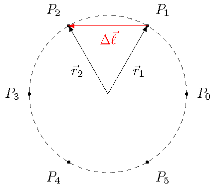
Fig. 27.4 Marked points and difference vectors for hexagon
Notice this method gives us a nice way to find the perimeter of any polygon! The next problem lets you try this, as a nice practice exercise. This would be an intermediate step for a final vPython program which calculates the magnetic field at the center of a circular loop.
Problem
Write a vPython function polyPerimeter() that calculates the perimeter of a polygon with \(N\) sides. Choose the corners of the polygon so that they are on a circle with radius \(R\), as described above. Add up the magnitudes of the vector differences \({\vec r}_{k + 1} - {\vec r}_k\) to get the total perimeter. Thus, the function polyPerimeter() should have two arguments: the number of sides N for the polygon, and the radius R of the circle where the corners are chosen. The function should return the perimeter of the polygon.
Show that, as \(N\) gets large, the perimeter of the polygon approaches the value \(2 \pi R\).
Answer: Here is a possible vPython program to solve the problem.
def polyPerimeter(N, R):

    # Definitions

    DQ = (2 * pi) / N            # Angle between adjacent points
    perimeter = 0                # Initialize perimeter variable

    for iii in range(N):
        vec_diff = R * vector(cos((iii + 1) * DQ), sin((iii + 1) * DQ), 0) - \
                    R * vector(cos(iii * DQ), sin(iii * DQ), 0)
        perimeter += mag(vec_diff)

    return perimeter
Now, let’s get back to solving the original problem. We want to use the unit vector \({\hat r}\) instead of the position vector \({\vec r}\), so dividing \({\vec r}\) by its magnitude \(R\), we have \({\hat r} = (\cos \theta) {\hat x} + (\sin \theta) {\hat y}\). Finally, remember I am using \(-{\hat r}\) instead of \({\hat r}\), since I defined the original vector \({\vec r}\) backwards. Thus, finding the contribution from a single side with the Biot-Savart law,
With the trigonometric identity \(\sin^2 \theta + \cos^2 \theta = 1\), this gives
Finally, let’s add up the contributions to get the total magnetic field. As we talked about above, we really want to take the limit with a very large number of sides \(N\), so
So what does this limit mean? Well, if the number of sides increases, then the sum of all the side lengths \(\sum \Delta \ell\) is going to approach the circumference \(2 \pi R\) of the circular loop! Hopefully you tried this limit when you wrote the vPython function polyPerimeter() in the problem above. This means that when we take the limit,
This gives us our first magnetic field calculation using the Biot-Savart law.
Magnetic field at the center of a circular loop
For a circular loop with radius \(R\), and current \(I\) moving through it, the magnitude \(B\) of the magnetic field at the center of the loop is given by
Notice that one factor of \(R\) has cancelled out, so the field magnitude depends on \(1/R\), not \(1/R^2\) – doubling the size of the loop only decreases the magnetic field by one-half, rather than one-fourth, as we might expect from the Biot-Savart law.
Problem
Suppose a circular loop of wire is lying in the \(x-y\) plane. It has a radius of 3.00 cm and a current of 1.25 A passing through it, in a clockwise direction as seen by you looking down on the loop from the \(+z\) direction. What is the magnetic field (in \(\mu\)T) at the center of the loop, due to the current?
Answer: \({\vec B} = (-1.31 \ \mu\textrm{T}) {\hat z}\)
27.5. Magnetic field due to a long, straight wire
In the last section, we derived the magnetic field at the center of a circular loop, by dividing the loop into small pieces \(\Delta {\vec \ell}\), and then adding up the magnetic field contributions \(\Delta {\vec B}\) from each of these pieces. Now we’ll turn to the magnetic field created by a long, straight wire. Here, “long” just means that the total length of the wire is large compared to the radius of the circular wire itself.
Solving for the magnetic field at a point \(P\) some distance away from a long, straight wire is more complicated than that for the circular loop, so I will just sketch the method you can use here. Much like the circular loop, you can divide the straight wire into smaller segments \(\Delta \ell\), and find the magnetic field contribution \(\Delta {\vec B}\) from each of these segments. The sum of these would then give the total magnetic field. However, unlike the loop, each of these contributions \(\Delta {\vec B}\) is not the same, for two reasons. First, the distances from the point \(P\) to each segment will be different, as you move further away from \(P\) along the wire. As you do this, you will also have the fact that the vector product \(\Delta {\vec \ell} \times {\hat r}\) is different for different segments; basically, the angle between the two vectors changes at different locations along the wire. Taking care of these aspects requires either a somewhat involved vPython program, or else integral calculus!
So let’s do this a much easier way – we can guess the form of the final \({\vec B}\) for a long, straight wire, and see why it is true, starting from the Biot-Savart law. This relation tells us that \({\vec B}\) should be proportional to \(\mu_0\) and \(I\). If we look at the units of the rest, \({\hat r}\) is unitless (remember we divide \({\vec r}\) by its magnitude). The remaining pieces are \(\Delta \ell\) and \(r^2\), which gives units of 1/length. Since the wire is infinite, the only relevant length is the distance \(R\) between the wire and the observation point \(P\). Thus, we expect that the magnitude \(B\) is given by
where \(k\) is some constant number. Going through the necessary integral calculus, you can show the following.
Magnetic field of a long, straight wire
The magnitude of the magnetic field at a distance \(R\) from a long, straight wire with current \(I\) is given by
Be careful! The field for the circular loop looks very similar, but its the one without the \(\pi\); the long, straight wire is the one with the \(\pi\). The geometric \(\pi\) coming from the circle cancels the \(\pi\) in the Biot-Savart law, which is why it does not appear in loop field equation.
Problem
A very long wire carries a current of 3.57 A to the right, as shown in the figure below.
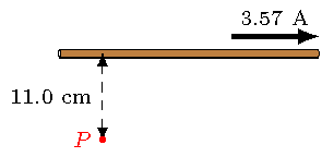
Fig. 27.5 A current-carrying wire
What is the magnitude and direction of the magnetic field at point \(P\)? Give the magnitude in \(\mu\)T.
At what distance (in cm) from the wire is the magnetic field strength equal to 5.00 \(\times 10^{-5}\) T?
Answers: \(6.49 \ \mu\)T, into the page; 1.43 cm
Problem
Two straight wires run parallel to each other, carrying currents in the amounts and directions shown. Which choice gives the net magnetic field strength at point \(P\) due to these two current carrying wires?
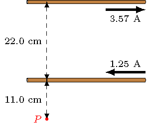
Fig. 27.6 Two parallel current-carrying wires
\(1.09 \times 10^{-7}\) T
\(2.16 \times 10^{-6}\) T
\(2.27 \times 10^{-6}\) T
\(4.44 \times 10^{-6}\) T
None of the above
Answer: \(1.09 \times 10^{-7}\) T
Problem
One of the long, straight wires shown below carries a current of 6.20 A in the positive \(y\) direction, and the second has a current of 4.50 A in the positive \(x\) direction.
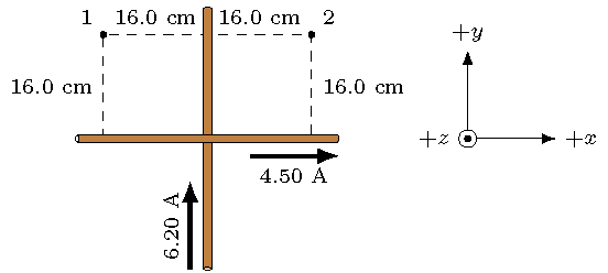
Fig. 27.7 Two crossed current-carrying wires
Calculate the net magnetic fields at points 1 and 2 in unit vector notation, using \(\mu\)T.
Answer: \({\vec B_1} = (13.4\ \mu\textrm{T}) {\hat z}\); \({\vec B_2} = (-2.13\ \mu\textrm{T}) {\hat z}\)
27.6. Summary
We have now talked about the sources of magnetic fields, which are all variations on current-carrying wires. Unlike the electric field (where the sources were just charges), the resulting magnetic fields are more complicated. This comes from the three-dimensional nature of the Biot-Savart law, as opposed to the simpler electric field equation due to a point charge. Hopefully you are getting some good practice with the vector product!
To emphasize the point, magnetic fields are created by the motion of electric charge: something electric is changing to give something magnetic. This relationship was shown to work both ways, which is why we now think of “electromagnetism”, rather than “electricity” and “magnetism” separately. This deep marriage of the two will continue in the next lesson, where we turn to Faraday’s law. This law relates the change of electric fields in space to produce changes in magnetic fields in time. It is because of such relations that we have light waves!
After this lesson, you should be able to:
State the magnitude and direction of the magnetic field due to a current-carrying wire.
Calculate the magnetic field at the center of a circular loop.
Calculate the magnetic field due to a long, straight wire.