13. Scalar product
13.1. Overview
Links to programs in this lesson:
There are many times where a mathematical object allows us to greatly simplify a calculation, where it would be tedious otherwise. Hopefully, you have seen that this is true with vectors – they nicely codify many physical properties in three dimensions, and summarize this information in one equation (rather than three!). So, as we have recently seen, all the possible situations in relation motion are condensed into two vector equations.
A similar idea motivates the definition of the “scalar product”. A major use of the scalar product for us will be identifying the angle between two vectors, and specifically when they are parallel or perpendicular. The scalar product will be used several times in the rest of the course. In Lesson 14, it helps define unit vectors for describing motion along a ramp, or perpendicular to it. In Lesson 19, the notion of “work” – defined as a scalar product between force and displacement – will be our gateway into the powerful methods of energy conservation.
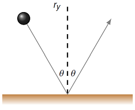
Fig. 13.1 Squash ball bouncing off of wall
To motivate the scalar product, let’s consider an example we looked at before. Suppose we have a ball bouncing against a wall, where the wall is along the \(x\) axis; this is shown in the figure above, taken from Lesson 10. We found there what is hopefully intuitive: the force of the wall does nothing to the \(x\) component of the ball’s velocity, but reverses the direction of the \(y\) component, keeping its size the same.
Notice that the same thing would happen if the wall were replaced by another ball! So this is a special example of a 2D collision. Now the question arises, what if the wall were not along the \(x\) axis, but at some arbitrary angle? How do we “reverse the direction” of only one of the ball’s velocity components? This is what would occur in a general 2D collision. You could work out the new velocity for any orientation of the wall, but it would be a trigonometric hassle. Instead, we can use the scalar product to find the perpendicular piece of the incoming velocity. This is an example of how we will be using this mathematical machinery. So, let’s now define the scalar product, and see it in action.
Here are the objectives for this lesson:
Calculate the scalar product of two vectors.
Given a vector \({\vec V}\), find a second vector that is perpendicular to \({\vec V}\).
Given a vector \({\vec V}\) and a set of vector equations, find the equation for the components parallel to \({\vec V}\), and the equation for the components perpendicular to \({\vec V}\).
13.2. Why the scalar product?
As we have seen in physics class, there are several times where mathematical tools are necessary to properly explain and understand physics concepts. For example, so far, you have seen trigonometry and vectors. These have helped us describe the motion of projectiles, see what happens when objects collide, and understand how moving objects appear to one another.
Focusing on vectors, up to this point, you have seen how to add and subtract vectors (vector addition) and to make them bigger or smaller in size (scalar multiplication), possibly flipping their direction 180\(^\circ\) at the same time. Is there anything else we can do with vectors?
It turns out that, given two vectors, there are two other mathematical operations we will see in this course. The first is called the scalar product (although often I will say “dot product”, because of the symbol used!), which takes two vectors \({\vec A}, {\vec B}\) and outputs a scalar \({\vec A} \cdot {\vec B}\).
Pay attention to the name
The scalar product gives you a scalar, not a vector!
As with all math ideas we use in this course, the scalar product is helpful in summing up an important physical idea: how much of one vector points along the same direction as the second vector. Notice that this idea is symmetric, since it doesn’t matter which vector in the scalar product you make the “first” or “second” in the previous sentence.
The scalar product will be useful for two things. First, given a vector \({\vec V}\), you can use it to find a second vector that is perpendicular to \({\vec V}\). Also, given a vector \({\vec V}\) and a vector equation, the scalar product allows you to find the components of that equation parallel to \({\vec V}\) (we have already done this secretly!)
You will see at different points that this gives you important information about the physics in a particular situation. In the next lesson after this one, we will use the scalar product to find the motion of a block along a ramp (or inclined plane) by separating the forces that are parallel and perpendicular to the incline. Later on, you will see the scalar product when we find the work done on an object by a force; this will be the first step in finding the mechanical energy of the object as it moves along.
There is a second operation, we will see the vector product (or “cross product”, again from the sign used to denote the operation), which takes two vectors and outputs a third vector that is perpendicular to the first two. We will see this in Lesson 17.
13.3. Definition of scalar product
The easiest way to define what the scalar product does to the two vectors involved is to see what it does to the unit vectors \({\hat x}, {\hat y},\) and \({\hat z}\) that point along each of the three axes. Remember that any vector in three-dimensional space can be written as the vector sum of scalar multiples of these vectors. It will be easy to see this, since the scalar product is defined so that it “strips off” the components of the vector. For example, if you have an arbitrary vector \({\vec A}\), then it can be written as the vector sum
where \(A_x, A_y,\) and \(A_z\) are its three components. If we take the scalar product of this vector with the unit vector \({\hat x}\), say, then the resulting scalar is just the \(x\) component of the vector!
The same would hold true for the other two components – the scalar product \({\vec A} \cdot {\hat y}\) would give the \(y\) component \(A_y\), for example. Note that it does not matter in which order you write the vectors; this is important to remember, since when we get to the vector product later in the class, this will not be true!
So what definition is necessary in order for this to happen? Again, the idea is that the scalar product with a unit vector is “stripping off” the piece of the other vector in that direction. In other words, only the part of the vector \({\vec A}\) that is parallel to the unit vector remains. The unit vectors \({\hat x}, {\hat y}\) and \({\hat z}\) are all perpendicular to each other – each of the three has no component along the other two – so that a little bit of thought leads to the following definition.
Unit vector form of scalar product
Suppose you have two vectors \({\vec A}\) and \({\vec B}\), given in unit vector form, in terms of the unit vectors \({\hat x}, {\hat y}\), and \({\hat z}\). The scalar product \({\vec A} \cdot {\vec B}\) can be found using the definitions
and
as well as the fact that \({\vec A} \cdot ({\vec B} + {\vec C}) = {\vec A} \cdot {\vec B} + {\vec A} \cdot {\vec C}\). In other words, you can distribute the scalar product, as you would when you multiply two polynomials.
These relations define the scalar product, and the result for two generic vectors can be found from these. For example, by using distribution,
Problem
Write a vPython procedure scalarProduct() that takes two vPython vectors as arguments. It should return the scalar product, using the definition given above. Do this without using any built-in vPython functions, other than the standard mathematical operators!
Answer: Here is an example function.
def scalarProduct(vec1, vec2):
    return vec1.x * vec2.x + vec1.y * vec2.y + vec1.z + vec2.z
Problem
Find the scalar product of the two vectors \({\vec F} = -3 {\hat x} + 5 {\hat y} + 6 {\hat z}\) and \({\vec G} = -2 {\hat x} + 4 {\hat y} - {\hat z}\).
Answer: The scalar product \({\vec F} \cdot {\vec G} = 20\).
Problem
Can the scalar product ever be negative? Zero? See if you can find two vectors \({\vec G}\) and \({\vec H}\) that have \({\vec G} \cdot {\vec H} < 0\), or \({\vec G} \cdot {\vec H} = 0\).
Answer: As two easy cases, the vectors \({\vec H} = {\hat x}, {\vec J} = -{\hat x}\) have scalar product \({\vec H} \cdot {\vec J} = -1\), while with \({\vec K} = {\hat y}\), then \({\vec H} \cdot {\vec K} = 0\). The geometric meaning of these cases will be explained below.
13.4. The scalar product in vPython
You can easily calculate the scalar product of two vectors in vPython – you can simply write dot(Avec, Bvec) for previously defined vectors Avec and Bvec. An example is shown below.
Problem
In the space provided in the app above, create two arrow objects Arr and Barr, with positions Arr.pos and Barr.pos at the origin, and axes Arr.axis and Barr.axis given by aVec and bVec, respectively. Notice the relative direction of the two arrows. Then, change the vectors Avec and Bvec to have the vector components you found for the last problem, where the scalar product was negative or zero. Do you notice a relationship between the value of the scalar product, and the relative directions of the two vectors?
Answer: Here is some example code that will create the arrow objects.
Aarr = arrow(pos = vector(0, 0, 0), axis = Avec, color = color.red, \
             shaftwidth = 0.1)
Barr = arrow(pos = vector(0, 0, 0), axis = Bvec, color = color.blue, \
             shaftwidth = 0.1)
As you remember from previously in the class, there are two ways to describe a vector: either in terms of its components (which we just saw above), or in terms of a magnitude and direction. We will now define two vectors using the latter method, and build up more intuition about the scalar product.
One way to define vectors is in terms of their magnitudes and angle. We will stick to the \(x-y\) plane so it does not get too complicated. This means that the only two vector components will be the \(x\) and \(y\) components of the vector, while the \(z\) component will be zero. In this case, a vector \({\vec V}\) with magnitude \(V\) (the variable V in Python) and angle \(\theta\) (I will use the variable Q for this) would be defined as
V = vector(V * cos(Q), V * sin(Q), 0)
Remember that the variable Q will be between zero and \(2 \pi\) radians, while the magnitude V must be positive!
The next program find the scalar product of two vectors, defined in terms of their magnitudes and directions, rather than their unit vector form. You will need to add the appropriate code that takes the magnitudes and angles, and finds the correct components.
Problem
In the program below, two magnitudes R and S are given, along with the angles Q_R and Q_S in radians. Define the vectors Rvec and Svec in vPython, and then run the program to calculate their scalar product.
Answer: To define the vector objects Rvec and Svec, one possibility is to use the commands
Rvec = R * vector(cos(Q_R), sin(Q_R), 0)
Svec = S * vector(cos(Q_S), sin(Q_S), 0)
Then, the scalar product \({\vec R} \cdot {\vec S} = 5.43537\).
Problem
In the program above, keep the angles the same, and change the magnitude of one of the two vectors. What happens to the scalar product? Does the scalar product ever become zero? Negative?
Problem
Now put the magnitudes back to their original values of \(R = 5\) and \(S = 3\), and change the angle of one of the two vectors. What happens to the scalar product now? Does the scalar product ever become zero? Negative? If you want, you can import the vPython module pi if you want to define your angles using a multiple of \(\pi\).
13.5. Geometry of the scalar product
Hopefully you have found that changing the magnitudes of the vectors only changes the size of the scalar product – the sign stays the same. However, if you change the angles, you can change both the size and the sign of the scalar product. What is going on?
The picture below helps us understand the scalar product of two vectors \({\vec A} \cdot {\vec B}\).
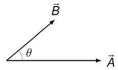
Fig. 13.2 Finding the scalar product of two vectors
For this illustration, we have done the following (much like what you just did in vPython!). I chose the \(+x\) axis so that it points along the first vector \({\vec A}\), and the \(+y\) axis so that the second vector \({\vec B}\) is in the \(x-y\) plane. This means that \({\vec A} = A {\hat x}\) and \({\vec B} = (B \cos \theta) {\hat x} + (B \sin \theta) {\hat y}\). Using the rule for the scalar product, \({\vec A} \cdot {\vec B} = AB \cos \theta\). This gives us a second definition for the scalar product.
Magnitude-angle definition of scalar product
Given two vectors \({\vec A}\) and \({\vec B}\), the scalar product of these vectors is
where \(A, B\) are the magnitudes of the vectors \({\vec A}, {\vec B}\), respectively, and \(\theta\) is the angle between the two vectors.
Thus, as we said at the beginning, the scalar product depends on the magnitudes \(A\) and \(B\) of the two vectors, as well as the angle \(\theta\) between them. If you made your two vectors above have a negative scalar product, it was because \(\cos \theta < 0\), while \(\cos \theta = 0\) gives a zero scalar product.
Problem
What range of angles \(\theta\) gives you \(\cos \theta < 0\)? What angles give you \(\cos \theta = 0\)? How would you describe the relative orientations of these vectors in each of those two situations?
Answer: \(\cos \theta < 0\) when \(\pi / 2 < \theta < \pi\) (in radians), and \(\cos \theta = 0\) when \(\theta = \pi / 2\).
Problem
Using the picture below, how does the value \({\vec A} \cdot {\vec B}\) change does the angle \(\theta\) increases in size?
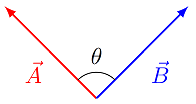
Fig. 13.3 Changing the angle \(\theta\) between two vectors
The value decreases in size.
The value increases in size.
The value stays the same.
Answer: Increasing the angle decreases the size of \(\cos \theta\), which has a maximum value of 1 when \(\theta = 0\).
Problem
Rank the pictures shown below according to the size of the value \({\vec A} \cdot {\vec B}\). Assume that all vectors have the same magnitude. Give your answer using the “\(<\)” and “\(=\)” signs, and the letters for each choice. For example, a possible answer would be “\(A = B < C < D\)”.
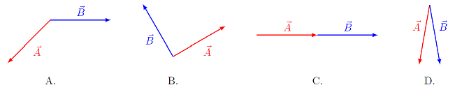
Fig. 13.4 Changing the angle \(\theta\) between two vectors
Answer: \(C > D > B > A\)
Problem
Suppose you are given a vector \({\vec A} = 4 {\hat x} - 7 {\hat y}\), shown in the diagram below.
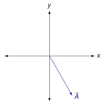
Fig. 13.5 Finding a vector perpendicular to a given vector
Review: Find the unit vector \({\hat A}\) in the same direction as \({\vec A}\).
Suppose you want to find a second vector \({\vec B} = B_x {\hat x} + B_y {\hat y}\) that is perpendicular to \({\vec A}\). What equation must be true for the two components \(B_x\) and \(B_y\)?
Using this equation, find a unit vector \({\hat B}\) in the first quadrant that has unit magnitude and is perpendicular to \({\vec A}\).
Answer: \({\hat A} = (4 / \sqrt{65}) {\hat x} - (7 / \sqrt{65}) {\hat y}\); \(4 B_x - 7 B_y = 0\); \({\hat B} = (7 / \sqrt{65}) {\hat x} + (4 / \sqrt{65}) {\hat y}\)
Problem
Above, you were given two vectors \({\vec F} = -3 {\hat x} + 5 {\hat y} + 6 {\hat z}\) and \({\vec G} = -2 {\hat x} + 4 {\hat y} - {\hat z}\). What is the angle between these two vectors (in degrees)?
Answer: The angle between \({\vec F}\) and \({\vec G}\) is 1.022 radians, or \(58.6^\circ\).
13.6. Breaking a vector into components
Now that we have gone through the idea of the scalar product, let’s see it in practice, by using it to find the components of vectors. Up until this point, I have just “read off” what is in front of all the \({\hat x}\) unit vectors, and said that gives the equations for the \(x\) components, for example. However, now we can be more formal about it. This will help in the next lesson, when we look at inclined planes. In those cases, it may be advantageous to use a perpendicular set of unit vectors other than \({\hat x}, {\hat y}\). Then, having a more rigorous way of finding each of the component equations is helpful.
To set up the situation, I will use the vectors shown in the figure below. The vector \({\vec C}\) is along the \(x\) axis, and \({\vec B}\) is along the \(y\) axis, while \({\vec A}\) is off at some angle in the second quadrant. For now, I have just labeled these as three vectors, but you can imagine this as a FBD; in fact, you will see this as a FBD in an example in the following lesson.
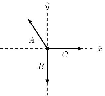
Fig. 13.6 Three vectors
First, let’s suppose that the three vectors add up to the zero vector, i.e.
Suppose we know the magnitudes \(B\) and \(C\), and are trying to find the third magnitude \(A\). I have drawn the vectors in the picture above to suggest using the standard \({\hat x}\) and \({\hat y}\) unit vectors to break down these vectors, and solve. In fact, doing it this way turns out to be easy. The known vectors are written as
so our vector equation becomes
Now, rather than just “reading off” the components as we have done before, I will use the scalar product to pull off the relevant components. In particular, if I take the scalar product of the last equation with \({\hat x}\), I get
The zero in the middle is because \({\hat y} \cdot {\hat x} = 0\); the last term \(C\) comes from \({\hat x} \cdot {\hat x} = 1\). Since \({\vec A} \cdot {\hat x}\) is just the vector component \(A_x\), then we get \(A_x = -C\). If instead, I take the scalar product of the original equation with \({\hat y}\), I get
where I have already written \({\vec A} \cdot {\hat y} = A_y\). This gives \(A_y = B\), and we now can describe \({\vec A}\) in terms of the magnitudes for the other two vectors as \(A = (-C) {\hat x} + B {\hat y}\).
This shows how to formally pull off the components in a vector equation, to get the individual component equations. At this point, you may wonder why I am going through all this, other than to make it more mathematical. Well, let’s change the problem a bit, so that the vectors no longer add up to the zero vector, and see what changes. Consider the diagram shown below. I have added a fourth vector \({\vec D}\) that is at an angle \(\theta\) to the \(+x\) axis, while \({\vec A}\) is now at the same angle away from the \(+y\) axis. Notice that this means \({\vec A}\) and \({\vec D}\) are perpendicular to each other, as are \({\vec B}\) and \({\vec C}\); this will be important later.
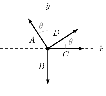
Fig. 13.7 Four vectors
You are given the magnitudes of the three vectors \({\vec A}, {\vec B}\), and \({\vec C}\), and we are looking for the magnitude \(D\). In addition, you are told that the following vector equation holds:
Again, I am keeping the situation a little vague, but you can imagine that this is a net force equation for an object on a ramp inclined at an angle \(\theta\) to the horizontal, and \({\vec D}\) is related to the acceleration of the object up the ramp.
Since I have kept the \({\hat x}\) and \({\hat y}\) labels for the axes, I will use those to find the components of each vector. The vector \({\vec B}\) and \({\vec C}\) are the same as above; I will write the other two as
We can go through the same process as before: start with the original vector equation written above, and take its scalar product with \({\hat x}\) and \({\hat y}\), respectively, to get the \(x\) and \(y\) component equations. This gives
Can you solve for the magnitude \(D\)? If you are seeing equations like these for the first time, it is probably not obvious what to do next!
Challenge
Solve the above equations for the magnitude \(D\), in terms of the magnitudes \(A, B\), and \(C\), and the angle \(\theta\). Hint: Multiply each equation by a different trigonometric function, and use the identity \(\sin^2 \theta + \cos^2 \theta = 1\).
Fortunately, there is an easier way to find \(D\), using a different set of coordinate axes. This will be helpful, since there are pairs of vectors that are perpendicular to each other. In particular, suppose I redraw the vector picture as shown below.
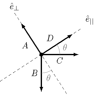
Fig. 13.8 Four vectors in a different coordinate system
Instead of using the usual unit vector \({\hat x}\) and \({\hat y}\), I now have \({\hat e}_{||}\) (as in “parallel to \({\vec D}\)”) and \({\hat e}_\perp\) (“perpendicular to \({\vec D}\)”). This is helpful for two reasons. The first is that \({\vec D}\) is obviously parallel to itself, so it will only have a component in the \({\hat e}_{||}\) direction. Also, \({\vec A}\) points in a perpendicular direction to \({\vec D}\), so it only has a \({\hat e}_\perp\) component. In other words, these vectors have unit vector notations given by
Notice this means we only need to consider the \({\hat e}_{||}\) component of the original vector equation to get \(D\)! The vector \({\vec A}\) will not factor in at all.
This simplification is balanced by the fact that the other vectors \({\vec B}\) and \({\vec C}\) have both parallel and perpendicular components. By the way, notice where the angles are for these vectors in the picture above. Since \({\vec B}\) and \({\vec C}\) are perpendicular to each other, the locations of the \(\theta\) are each to a different axis: between \({\vec B}\) and the \({\hat e}_\perp\) axis, and between \({\vec C}\) and the \({\hat e}_{||}\) axis. We can break these up into components as follows, using the individual vector diagrams below.
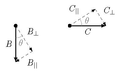
Fig. 13.9 Vector diagrams for \({\vec B}\) and \({\vec C}\)
Using these components, if we find the \({\hat e}_{||}\) of the master vector equation, we get simply
Problem
You are given the four vectors shown in the diagram below, where \({\vec E}\) is perpendicular to \({\vec F}\), and \({\vec G}\) and \({\vec H}\) are also perpendicular. There is an angle \(\theta = 35.0^\circ\) between \({\vec E}\) and \({\vec H}\). You are given the magnitudes \(E = 2.85\) and \(F = 6.70\). If the four vectors add up to the zero vector, solve for the magnitudes \(G\) and \(H\).
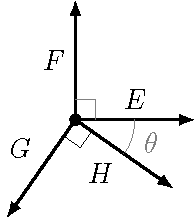
Fig. 13.10 Four vectors that add up to the zero vector
Answers: \(G = 7.12\), \(H = 1.51\)
13.7. Decomposing arbitrary vectors
I will finish this lesson by building on the scalar product, and the methods we just developed for finding vector components for arbitrary perpendicular unit vectors. Suppose we have two vectors \({\vec V}\) and \({\vec W}\) at some arbitrary angle between each other, and we want to break the vector \({\vec V}\) into two pieces – one parallel to \({\vec W}\) and the other perpendicular to \({\vec W}\). We will call these pieces \({\vec V}_{||}\) and \({\vec V}_\perp\), respectively. This is similar to what we did earlier, when we derived the relation \({\vec A} \cdot {\vec B} = AB \cos \theta\). How can we do this?
If \({\vec W}\) is along one of the coordinate axes, then this is relatively easy to do: we just write \({\vec V}\) in unit vector notation, and identify which of the components are along \({\vec W}\). For example, if \({\vec W} = W {\hat y}\), then the component \(V_y {\hat y}\) is along \({\vec W}\), and the rest of \({\vec V}\) is perpendicular. Let’s be pedantic here, and spell out exactly what is going on; this will help in the general case. Suppose we have vectors
An example would be \({\vec W}\) is the normal vector pointing away from a wall, and \({\vec V}\) is the velocity of a ball moving towards the wall.
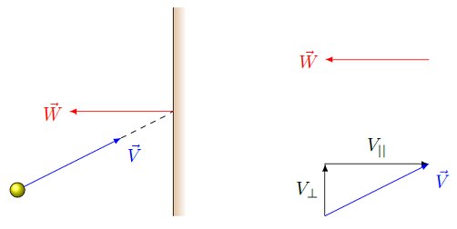
Fig. 13.11 Finding the components of velocity \({\vec V}\) relative to the normal vectors \({\vec W}\) for the wall
By the definition of vector components in terms of the scalar product,
so the vector parallel to \({\vec W}\) is
Then, since we want the vector sum of the components to add up to \({\vec V}\), or
this gives that the perpendicular component \({\vec V}_\perp\) is
Now, how do we make this general? Well, notice that the unit vector \({\vec y}\) in this specific case is just the unit vector \({\hat W}\) in the direction of \({\vec W}\)! This comes from our definition of the unit vector \({\hat W}\). Since the vector \({\vec W}\) only points in the \(y\) direction here, then the magnitude is just the \(y\) component, or \(W = W_y\).
Thus, we can rewrite the equations above as
This gives the vector decomposition of \({\vec V}\) into two pieces, the part \({\vec V}_{||}\) parallel to \({\vec W}\), and the second \({\vec V}_\perp\) perpendicular to \({\vec W}\). This works for any two vectors!
Problem
Below is a diagram with two vectors \({\vec A}\) and \({\vec B}\). The magnitudes and angles for each vector are \(A = 1.66, B = 2.87\) and \(\theta_A = 25.0^\circ, \theta_B = 15.0^\circ\). Give your answers to the problems below in unit vector form.
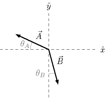
Fig. 13.12 Two vectors \({\vec A}\) and \({\vec B}\)
Find the unit vector \({\hat A}\).
Using this vector \({\hat A}\), find the vectors \({\vec B}_{||}\) and \({\vec B}_\perp\) that are parallel and perpendicular, respectively, to the vector \({\vec A}\). These vectors should satisfy the equation \({\vec B}_{||} + {\vec B}_\perp = {\vec B}\) and \({\vec A} \cdot {\vec B}_\perp = 0\).
Answers: \({\hat A} = -0.906 {\hat x} + 0.423 {\hat y}\); \({\vec B}_{||} = 1.67 {\hat x} - 0.780 {\hat y}\) and \({\vec B}_\perp = -0.929 {\hat x} - 1.99 {\hat y}\)
Problem
Write a vPython function vecComponents() which, given a first vector \({\vec W}\), finds the two vectors \({\vec V}_{||}\) and \({\vec V}_\perp\) such that (1) they add up to a second vector \({\vec V}\), i.e. \({\vec V}_{||} + {\vec V}_\perp = {\vec V}\) and (2) \({\vec V}_\perp \cdot {\vec W} = 0\). Thus, the two arguments of vecComponents() should be W and V, and the function should return a list made of two vectors vPar and vPerp (in that order), such that vPar + vPerp = V and dot(vPerp, W) = 0.
Answer: Here is a possible vPython program to break \({\vec V}\) into two vectors parallel and perpendicular to \({\vec W}\). You can use this program to test the answers for the previous problem.
def vecComponents(V, W):

    hatW = norm(W)             # Find unit vector in same direction as vector W

    vPar = dot(V, W) * hatW    # Find vector parallel to W
    vPerp = V - vPar           # Find vector perpendicular to W

    return [vPar, vPerp]
Challenge
Using algebra and the appropriate definitions, show that \({\vec V}_{||}\) is parallel to \({\vec W}\) by showing that \({\vec V}_{||} \cdot {\vec W} = {\vec V} \cdot {\vec W}\). Similarly, show that \({\vec V}_\perp\) is perpendicular to \({\vec W}\) by showing that \({\vec V}_\perp \cdot {\vec W} = 0\).
13.8. Isn’t this just “vector multiplication”?
One question I get asked a lot is whether this is all just “multiplying” vectors. To answer that, let’s think about what multiplication means. The simplest way to understand multiplication is to combine groups of objects. If I have two baskets, and each basket has three oranges in it, then I have \((2)(3) = 6\) oranges total. In other words, the total number of oranges is twice as big as the amount in each basket. Another way of thinking about multiplication is as the inverse of division. To say that \((2)(3) = 6\) means that I can divide 6 into two groups of three (\(6 / 2 = 3\)), or I can also divide it into three groups of two (\(6 / 3 = 2)\).
Now we return to vectors. First, when I think of “making a vector bigger”, what am I saying? If I have a vector \({\vec V}\), and make it twice as big, I can imagine this means making the magnitude \(V\) twice as big. But this is the idea behind scalar multiplication, where we multiply each component of the vector by the same scalar. I could also imagine that I “make the angle bigger”, but that quickly leads to weird thinking – if an acceleration vector has a magnitude of 3.00 m/s\(^2\) at 40.0\(^\circ\) west of south, and I triple it, is the new vector now at 120\(^\circ\) west of south? What does that mean? (It might help to try and draw a picture, to see that this description of an angle is not useful!)
If I turn to division, what does it mean to divide a vector by another? If I wanted to “divide” the vector \({\vec A}\) by the vector \({\vec B}\), I could guess that I divide the components of \({\vec A}\) by those of \({\vec B}\). But what if one of the components of \({\vec A}\) is zero? Or of \({\vec B}\)? Do I get a unique answer for this division, or are there multiple possibilities?
This is why the scalar product defined here is different than ordinary multiplication of numbers. We have seen that there are vectors whose scalar product is zero – those vectors must be perpendicular to each other. But we can’t imagine “undoing” the scalar product (as division “undoes” multiplication) in a case like that. It is not helpful to think of the scalar product as “multiplying vectors”, it is something different!
13.9. Summary
We now have defined the scalar product, a “mathematical machine” that takes two vectors and gives a number proportional to their magnitudes, and the cosine of the angle between them. This allows us to easily find out whether a pair of vectors are parallel or perpendicular, and to break a vector up into components. We will use the scalar product at different points in the course, starting with the next lesson, where we look at objects moving along a ramp.
After this lesson, you should be able to:
Calculate the scalar product of two vectors.
Find the angle between two arbitrary three-dimensional vectors.
Given a vector, find a second vector perpendicular to it.