17. Vector product
17.1. Overview
Links to programs in this lesson:
Suppose you have two vectors, and you want a mathematical operation that combines them to get a new quantity. By this, I mean that it doesn’t matter how you choose your coordinate system – the answer for these operations is independent of your choice. It turns out that, in any dimension, there are only two ways to do this, so that everyone agrees on the answer! The first of these is something we have already seen, the scalar product \({\vec A} \cdot {\vec B}\) of two vectors \({\vec A}\) and \({\vec B}\), defined in Lesson 09. If I use the unit vectors \({\hat x}\) and \({\hat y}\) (horizontal and vertical), while you are working with a ramp, so you use the unit vectors \({\hat e}_{||}\) and \({\hat e}_\perp\) (parallel and perpendicular) matching the ramp. It turns out that if you calculate the scalar product of two vectors using either possibility for the unit vector notation, you get exactly the same answer. Hopefully this makes sense, because the scalar product only depends on (1) the size of each vector, and (2) the angle between them. These values do not depend on how we orient our coordinate system. The scalar product was helpful in Lesson 14 (inclined planes) in finding a new set of unit vectors parallel and perpendicular to an inclined plane; it will also appear in Lesson 19 for the definition of the work done by a (constant) force.
In this lesson, we look at the only other way to define a quantity that is again the same, regardless of the coordinates used. This new mathematical operation is known as the vector product (or “cross product”). Like the name suggests, this will take two vectors and spit out a third vector. However, it will also have a geometric interpretation as well. It is this viewpoint that assures us that the vector product is independent of the coordinate choice.
Here are the objectives for this lesson:
Calculate the vector product of two vectors.
Use the right-hand rule to find the direction for the vector product.
Explain the properties of the vector product \({\vec A} \times {\vec B}\).
17.2. Rotational quantities as vectors
The vector product can appear to be odd at first glance, so before we get into its definition, let’s take a moment to see why it is useful. For now, it is going to be needed to deal with objects that are rotating. Unlike much of what we have done up to this point, rotations are inherently three-dimensional, so the physics and math we use needs to reflect this. First, we consider what a rotation does. Every rotation consists of two aspects:
a rotational axis about which the rotation occurs
a plane perpendicular to the axis, where all vectors in the plane are rotated around the axis (either CW or CCW)
The figure below shows how these attributes are related for a rotation axis along the \(z\) axis. These two aspects can be combined mathematically to a vector description of the rotation. Suppose we look at a small change \(\Delta \theta\) in angle counterclockwise about the \(+z\) axis. This rotates vectors in the \(x-y\) plane. In other words, the \(x\) and \(y\) coordinates of every point will change because of this rotation, while the \(z\) coordinate will remain the same. In the pictures below, the \(x-y\) plane is in the page, while the \(z\) axis points out at you.

Fig. 17.1 Every rotation axis has a plane perpendicular to it, where the rotation occurs
From this notion, we get that “rotation” = “axis + angle”. Thus, we can define a vector \(\Delta {\vec \theta}\) associated with a rotation of \(\Delta \theta\) around an axis. Again, in the right-hand picture above, the plane is in the page, and the vector \({\vec \theta}\) is pointing out at you. There are rotational versions of velocity and acceleration – namely, the angular velocity \({\vec \omega}\) (Greek letter “omega”) and the angular acceleration \({\vec \alpha}\) (Greek letter “alpha”). These are defined as you would expect:
The directions of these vectors is defined similar to that of \(\Delta {\vec \theta}\), perpendicular to the plane of rotation. Although thinking of an angular velocity or acceleration in a plane in terms of a vector perpendicular to the plane is strange at first, this will help explain many of the properties of rotational motion.
Much as there are rotational versions of the quantities displacement, velocity, and acceleration, there are also rotational versions of a force. These “torques” that produce angular accelerations, changing the angular velocity of an object. Suppose you have a rotating disk, as shown in the first picture below. The disk is rotating counterclockwise at a certain number of rotations per second, or its angular speed. This information (“CCW” + rotation rate) can be encoded in the vector \({\vec \omega}_i\). Its size gives the angular speed, and its direction tells us the rotation is counterclockwise. We will come back to the relationship between the direction of \({\vec \omega}_i\) and the rotation direction later in the lesson.
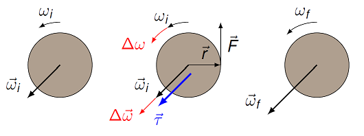
Fig. 17.2 A torque produces a change in the angular velocity of an object
Now, let’s have a force \({\vec F}\) acting on the outside edge of the disk, asw shown in the middle figure. This force will produce a torque \({\vec \tau}\) (Greek letter “tau”) on the object, changing its angular velocity \({\vec \omega}\) in size. For now, I will talk about torque conceptually; in Lesson 18 (angular momentum), I will define it more properly. In this situation, the torque is acting to increase the angular speed of the disk, i.e. the number of rotations per second is getting larger. Thus, the angular velocity vector will change from \({\vec \omega}_i\) to \({\vec \omega}_f\), where the two vectors are in the same direction, but \({\vec \omega}_f\) has a larger magnitude. A torque can also decrease the magnitude of the angular velocity, as shown in the next diagram.
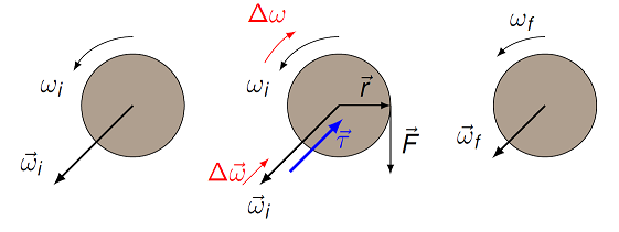
Fig. 17.3 A torque decreasing the magnitude of the angular velocity
We will now spend too much time talking about these quantities \({\vec \omega}\) and \({\vec \tau}\), but you may see them in another physics class. Just remember that these are vector quantities, even though they not be presented that way.
17.3. Vector product
17.3.1. The vector product in vPython
The vector product operation is inherently three-dimensional, so it may be difficult sometimes to see what is going on. Because of this, we are going to see what the vector product of two vectors looks like before we get into the mathematical definition. Hopefully doing it this way will increase your intuition of why the vector product is defined the way it is. As with the scalar product, there is a module in vPython that calculates the vector product for you. This module is known as cross, and its use is shown in the program below. Here, the same two vectors \({\vec A}\) and \({\vec B}\) saw when introducing the scalar product in Lesson 09 are defined, then their vector product \({\vec A} \times {\vec B}\) is calculated.
Remember that, for the same vectors, you found in Lesson 11 that the scalar product \({\vec A} \cdot {\vec B} = 1\). Obviously, for the vector product, the answer here is a vector, not a scalar. This vector points in the \(+z\) direction, since that is the only non-zero component. Also, the magnitude of the vector is \(|{\vec A} \times {\vec B}| = 7\), which is not the same as the value of the scalar product. So the vector product gives you different information about the relationship between the vectors than the scalar product did!
Now, let’s see what these vectors look like. The program below creates arrows for the two vectors \({\vec A}\) and \({\vec B}\), along with the vector \({\vec C} = {\vec A} \times {\vec B}\). In addition, it creates a box object called plane – this represents the flat surface in which the two original vectors \({\vec A}\) and \({\vec B}\) sit. Run the program, and see what you notice about the arrangements of the three vectors and the plane.
After you run the program, you will see the white vector \({\vec C}\) point straight out of the screen, in the \(+z\) direction. The other two vectors are embedded in the green plane; you should change your viewpoint to verify this. Notice also that the vector \({\vec C}\) is perpendicular to this plane, and therefore \({\vec C}\) is perpendicular to both \({\vec A}\) and \({\vec B}\).
Now let’s play around with these vectors a little.
Problem
Go back to the program above, and instead of letting the white arrow be \({\vec C} = {\vec A} \times {\vec B}\), change the vector product so that it is now \({\vec B} \times {\vec A}\). In other words, reverse the order of the two vectors inside cross. What happens to the white arrow? Does its magnitude change? Its direction?
When you did the last problem and ran the program, you should notice that \({\vec B} \times {\vec A}\) has the same magnitude as \({\vec A} \times {\vec B}\), but points in the opposite direction. In other words, as a vector equation
So the order in which you define the vector product is important!
Next, let’s see how changing the magnitude and direction of the two original vectors affects the final vector product. We define two vectors \({\vec R}\) and \({\vec S}\) in terms of their magnitudes R, S and direction angles Q_R, Q_S, keeping to the \(x - y\) plane so things are simple. Then we repeat the code from above, and see what the vector product \({\vec T} = {\vec R} \times {\vec S}\) looks like.
Problem
In the program below, define the two vPython vectors Rvec and Svec using the appropriate code. These commands should be in terms of the magnitudes R, S, and the angles Q_R, Q_S. Then run the program, and see what you get for the vector product of the two vectors.
Answer: One possible set of commands to define Rvec and Svec are given below.
Rvec = R * vector(cos(Q_R), sin(Q_R), 0)
Svec = S * vector(cos(Q_S), sin(Q_S), 0)
Problem
Without changing the directions of either vector \({\vec R}\) or \({\vec S}\), double the magnitude of one of the vectors. What happens to the magnitude and direction of the vector product \({\vec T}\)? What if you double both magnitudes?
Answer: The vector product is proportional to the magnitudes of the two vectors. Thus, doubling the magnitude of one of the vectors, with no other changes, will double the magnitude of the vector product, but the direction remains the same. Doubling the magnitude of both vectors simultaneously will quadruple the magnitude of the vector product.
Problem
Put the magnitudes back to their starting values \(R = 3\) and \(S = 2\). Now change the angles of the vectors, keeping the magnitudes the same. What happens to the magnitude and direction of the vector product \({\vec T}\)? When is the magnitude of \({\vec T}\) the largest? The smallest?
Answer: With fixed magnitudes, the magnitude of the vector product will be smaller when the angle is close to either zero degrees or 180.\(^\circ\). On the other hand, it is largest when the angle is around 90.0\(^\circ\). The direction remains the same as long as the different in angle between the vectors is less than 180.\(^\circ\). When the angle between the vectors exceeds this value, then you have gone from \({\vec R} \times {\vec S}\) to \({\vec S} \times {\vec R}\) (i.e. the order has reversed), and the direction of the vector product is opposite what it was before.
For whatever values you change the magnitudes and directions of \({\vec R}\) and \({\vec S}\) to, you will see that the vector product \({\vec T}\) is always perpendicular to the other two vectors. Here is a helpful way to think of the vector product of two vectors \({\vec A} \times {\vec B}\).
Geometry of the vector product
If the two vectors \({\vec A}\) and \({\vec B}\) are not parallel, they define a plane (shown in gray in the figure below). The vector \({\vec A} \times {\vec B}\) is perpendicular to both \({\vec A}\) and \({\vec B}\), so it is perpendicular to the plane as well.
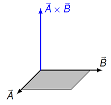
Fig. 17.4 The vector product \({\vec A} \times {\vec B}\) will always be perpendicular to the plane defined by two non-parallel vectors \({\vec A}\) and \({\vec B}\)
You might also have noticed a relationship between which way the two original vectors point versus the direction of their vector product. It turns out there is a rule you can use to determine this in situations where you know the directions of the original vectors. This rule is known as the “right-hand rule”:
Index finger straight out in direction of first vector \({\vec A}\)
Middle finger moved to point in direction of second vector \({\vec B}\)
Thumb will point in direction of \({\vec A} \times {\vec B}\)
Going from \({\vec A} \times {\vec B}\) to \({\vec B} \times {\vec A}\) means flipping your hand upside-down! You can see that in the diagram above – to flip the vectors \({\vec A}\) and \({\vec B}\), you should change the direction of the vector resulting from the vector product as well.
We can use the right-hand rule to see why the angular velocity \({\vec \omega}\) for the rotating disk we talked about above had the direction it did. For a disk rotating counterclockwise (as seen by you!), pick any point \(P\) on the disk, at a given position vector \({\vec r}\) araway from the disk’s center. At any particular time, the point \(P\) will be moving with a (linear) velocity \({\vec v}\). Then \({\vec r} \times {\vec v}\) will have the same direction as \({\vec \omega}\), in this case, towards you for a counterclockwise rotation.
17.3.2. Definition of vector product
Now we get into the mathematical definition of the vector product. From using the vPython code above, you should have found the following properties:
The vector product \({\vec A} \times {\vec B}\) is a new vector that is always perpendicular to the vectors \({\vec A}, {\vec B}\).
Because of how it is defined, the vector \({\vec A} \times {\vec B}\) has the same size, but points in the opposite direction to \({\vec B} \times {\vec A}\). This means \({\vec A} \times {\vec B} = -{\vec B} \times {\vec A}\).
Changing the magnitude of one of the vectors \({\vec A}\) or \({\vec B}\) will change the magnitude of \({\vec A} \times {\vec B}\) by the same factor. For example, if \({\vec A}\) is multiplied by a scalar \(k\), then \(|(k {\vec A}) \times {\vec B}| = k |{\vec A} \times {\vec B}|\).
Suppose the magnitudes of the two vectors \({\vec A}\) and \({\vec B}\) are kept the same. Their cross product will have the largest size when the vectors are perpendicular to each other, and will have a magnitude of zero when they are parallel (or \(180^\circ\) apart).
Like we did with the scalar product, we will define the vector product first in terms of the unit vectors along the coordinate axes. The vector product of a unit vector with itself gives the zero vector:
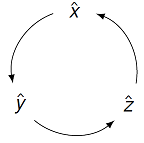
Fig. 17.5 Finding the vector product of the unit vectors
The vector product of two different unit vectors will give the third unit vector in the positive direction if the pair follows the cyclic patterns shown in the figure above. For example,
Reversing the order of the two vectors flips the sign of the vector product (going against the arrows):
Notice that just from these definitions, we have the first two properties of the vector product listed at the beginning of this section: perpendicularity, and flipping the order means flipping the sign. For the vector product of two general vectors, we can distribute using the rules for the unit vectors above to give
This equation is a little more complicated than the one for the scalar product, since we have three components to find, and it is important to be careful of the order in each one. However, you can see that the magnitude of the vector \({\vec A} \times {\vec B}\) depends on the magnitude of the individual vectors \({\vec A}\) and \({\vec B}\). For example, if you double the size of \({\vec A}\), this will also double the size of all its components \(A_x, A_y\), and \(A_z\), so then all the components of \({\vec A} \times {\vec B}\) will double in size as well.
Problem
Which choice below gives the vector product of the vectors \({\vec M} = -4 {\hat x} + 5 {\hat y}\) and \({\vec N} = -6 {\hat x} - 9 {\hat y}\)?
\(-21 {\hat z}\)
\(-15 {\hat z}\)
\(+6 {\hat z}\)
\(+66 {\hat z}\)
\(+135 {\hat z}\)
Answer: \(+66 {\hat z}\)
Problem
Compute the vector products of the following pairs of vectors (in the order they are given!).
\({\vec A} = -5 {\hat y} + 9{\hat z}\) and \({\vec B} = -{\hat y} - 5{\hat z}\)
\({\vec C} = 4 {\hat x} - 2{\hat z}\) and \({\vec D} = 7{\hat x} - 3{\hat z}\)
\({\vec E} = -2 {\hat x} - 7{\hat z}\) and \({\vec F} = 7{\hat x} + 7{\hat y}\)
\({\vec G} = -6 {\hat x} + 3{\hat y} + 2{\hat z}\) and \({\vec H} = 9{\hat x} + 7{\hat y} - 9{\hat z}\)
Answers: \({\vec A} \times {\vec B} = 34 {\hat x}\); \({\vec C} \times {\vec D} = -2{\hat y}\); \({\vec E} \times {\vec F} = 49 {\hat x} - 49{\hat y} - 14{\hat z}\); \({\vec G} \times {\vec H} = -41 {\hat x} - 36{\hat y} - 69{\hat z}\)
Problem
Verify your answers for the last two problems by using the cross module in vPython, along with the appropriately defined vectors.
Challenge
Although the vector products of each of the unit vectors with each other are perpendicular, this does not guarantee that a sum of unit vectors will be perpendicular as well. Using the definition given above, prove that \({\vec A} \times {\vec B}\) is perpendicular to both \({\vec A}\) and \({\vec B}\). Remember that you can use the scalar product of two vectors to show whether they are perpendicular or not.
17.3.3. Magnitude of vector product
Just like we did for the scalar product, we can write the magnitude \(|{\vec A} \times {\vec B}|\) of the vector product can be written in terms of the magnitudes \(A\) and \(B\) as well as the angle \(\theta\) between them. This can be proven by aligning the two vectors \({\vec A}\) and \({\vec B}\) to make it clear.
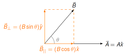
Fig. 17.6 Finding the vector product of the unit vectors
First, I will choose the first vector \({\vec A}\) to be along the \(+x\) axis, so \({\vec A} = A {\hat x}\)., Then, I pick the \(+y\) axis so the second vector \({\vec B}\) is in the first quadrant, and choose the \(z\) axis so that \(B_z = 0\). I can break up \({\vec B}\) into its components parallel and perpendicular to \({\vec A}\) (i.e. the \(x\) and \(y\) components, respectively); I will call these \(B_{||}\) and \(B_\perp\), respectively. Since
then the magnitude of the vector product is given by
This gives us a nice equation for the magnitude of the scalar product of two vectors. Compare this to the scalar product \({\vec A} \cdot {\vec B} = AB \cos \theta\). Both depend on the magnitudes of the individual vectors, so (as we saw earlier) changing one of the magnitudes by some factor will change the magnitude of \({\vec A} \times {\vec B}\) by the same factor. Also, \(|{\vec A} \times {\vec B}|\) depends on the angle \(\theta\) between the two vectors, but is now the sine, rather than the cosine, function.
Problem
Starting with the situation shown in the picture below, how does the magnitude \(|{\vec A} \times {\vec B}|\) change as the angle \(\theta\) decreases in size? Choose the best answer.
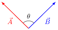
Fig. 17.7 Changing the angle \(\theta\) between two vectors
The value decreases in size.
The value increases in size.
The value stays the same.
Answer: The value \(|{\vec A} \times {\vec B}|\) will decrease in size, since the two vectors are becoming more aligned with each other.
Problem
Rank the pictures shown according to the size of the value \(|{\vec A} \times {\vec B}|\). Assume that all vectors have the same magnitude. Give your answer using the “\(<\)” and “\(=\)” signs, and the letters for each choice. For example, a possible answer would be “\(A = B < C < D\)”.
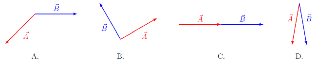
Fig. 17.8 Ranking the size of the vector product
Answer: \(C < D < A < B\)
Problem
The magnitudes of the vectors shown below are \(R = 8.54, S = 8.60\), and the angle \(\theta = 165^\circ\). What is the magnitude of \({\vec R} \times {\vec S}\)?
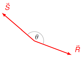
Fig. 17.9 Find the magnitude of the vector product \({\vec R} \times {\vec S}\)
Answer: 19.0
Combining together the right-hand rule (from the last section) and the magnitude formula \(|{\vec A} \times {\vec B}| = AB \sin \theta\), we can find the vector form of the vector product.
Problem
Find the vector products given below and give your answers in unit vector notation. The magnitudes of the three vectors shown are \(T = 2.45, V = 3.30\) and \(W = 4.05\).
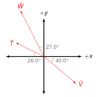
Fig. 17.10 Find the vector product for each pair of vectors
\({\vec V} \times {\vec W}\)
\({\vec T} \times {\vec W}\)
\({\vec T} \times {\vec V}\)
Answers: \({\vec V} \times {\vec W} = 5.22 {\hat z}\); \({\vec T} \times {\vec W} = -5.97 {\hat z}\); \({\vec T} \times {\vec V} = 1.96 {\hat z}\)
17.4. Vector products using matrices
Another way to compute the vector product of two vectors is to use matrices. A matrix is a rectangular block of numbers put into rows and columns. You may see these later on for solving simultaneous equations in a matrix algebra class, and they have a wide variety of uses – from engineering and physics, through computer graphics in TV and movies, to finding the best search results in Google. If you are interested in learning more about matrices, and what their determinant means, there is a great series of videos here, made by one of my favorite YouTube vloggers.
For now, all we need is to find a quantity known as the determinant. We will not do the general case, since all we need to know is how to find it for a square matrix with three rows and columns. The general pattern is similar to what we do here, though.
Suppose we have two vectors \({\vec A}\) and \({\vec B}\) with components
We will show that the vector product can be written as
There are different ways of evaluating this determinant, but the way I prefer to use is to do the following. Copy the last two columns, and repeat them at the end of the matrix. Then it now looks like
Start at the \({\hat x}\) in the top left corner of the matrix, and multiply everything along the diagonal pointing down and to the right. Subtract from this what you get by starting at the copied \({\hat x}\), and multiplying everything along the diagonal pointing down and to the left. This gives the \(x\) component of the vector product,
Do the same for the other two unit vectors. Note that for \({\hat z}\), you will start at the same place, but add the diagonal going down and to the right, and subtract the diagonal going down and to the left. When you add all the terms together, you get the vector product we found earlier:
Doing it this way for full three-dimensional vectors can help keep track of all your components. You may find it more useful than distributing like we did above.
17.5. Summary
The vector product is a strange beast the first time you see it, since it probably does not behave the way you expect it to! We will see the vector product again several times in the rest of the course, so it is a good idea to get the basics down now. It is part of the definition of angular momentum in the next lesson. It also appears in magnetism, where you may have previously encountered the “right-hand rule” for the magnetic force. As we will see, this magnetic force is inherently three-dimensional because of the vector product.
After this lesson, you should be able to:
Calculate the vector product of two given vectors.
Describe the properties of the vector product in relation to the original vectors.
Calculate the magnitude of the vector product.
Describe how the vector product changes depending on the angle between the original vectors.