20. Conservation of energy
20.1. Overview
Links to programs in this lesson:
In the last lesson, we found the work done by any generic force, as the system it acts on undergoes a displacement. This force could be constant (such as the force of gravity near the surface of the Earth) or changing (like the spring force). However, this is not the best way to divide forces, at least when talking about work. Instead, we will see that it is best to focus on those forces where the work done by the force leads to a scalar uniquely defined at every state of the system. This scalar will be known as a potential energy of the force, and the force will be known as a conservative force. The reason to do this is that if we can associate a specific scalar – the mechanical energy of the system – based on both kinetic and potential energies, then a constant mechanical energy allows us to predict the evolution of the system.
So our gameplan for this lesson is the following. First, we discuss which forces we can define potential energies for. There are a limited number of such forces, but they will be very helpful to use. This means we need to specify the difference between a conservative force and a non-conservative force; a potential energy can only be defined for a conservative force. Then we can add up the kinetic energy and all the potential energies of the system to get the system’s mechanical energy. If only conservative forces act on the system, then the mechanical energy is conserved, according to the work-energy theorem of the last lesson. However, if we have non-conservative forces as well, we need to take these into account. That will be the final portion of this lesson.
Here are the objectives for this lesson:
Define potential energy, and describe its relation to the force done by a conservative force.
Define mechanical energy, and explain when mechanical energy is conserved for a system.
Use the conservation of energy equation to solve for an unknown quantity in a system.
Describe the relationship between mechanical energy and the work done by non-conservative forces.
Use the conservation of energy equation to solve for an unknown quantity in a system, when non-conservative forces are present.
Given an energy graph for an object, describe the motion of the object.
20.2. Conservative vs. non-conservative forces
As outlined in the last section, our first step is to see where we can define a potential energy. Before we do that, let’s motivate why we can do that in the first place! For some forces, the work done by that force can be “stored” in the system. To see what that means, imagine that you have a person skating on a frictionless surface. You can see this by running the PhET app below, selecting “Intro”, and then moving the person onto the ramp and letting go. The skater will then move along the ramp.
If you watch the motion of the skater, you will see that they will continue moving forever. When they start at the top of the ramp, the gravitational force will pull them along the ramp, and they will speed up until they reach the bottom. At that point, as they start moving up the opposite side, gravity will slow them down, until they reach the same height again. But there is no friction, so this process will repeat itself over and over! There is some physical quantity related to gravity that is lost when the skater moves down the ramp, but is gained back in full when going back up the other side.
Let’s make this idea more general by considering some unknown force \({\vec F}\) acting on an object. Suppose you take the object and you move it from point \(a\) to point \(b\) in the figure below, using the long path with the green arrow. You find that the unknown force does 60 J of work on the object. Then you use the shorter path (the red arrow) to move the object back from point \(b\) to point \(a\). In this case, the force does -60 J of work.
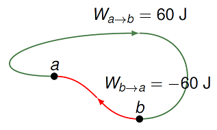
Fig. 20.1 The amount of work done by a force may depend on the path taken
Traveling from \(a\) to \(b\) you must put 60 J of work into the system due to a force \(F\) (“storage”), while from \(b\) to \(a\), 60 J of energy is taken out of the system due to force \(F\) (“release”). Said a different way, there is no change in the energy of the object when it takes a full cycle around the two arrows. This means for this force, there is some quantity that remains the same, regardless of how you go along the path. If we go against the arrows, then the signs of the works flip, but we still get the same net work of zero.
This force is known as a conservative force. A conservative force is one where the work done by the force on an object does not depend on the path taken by the object, for given initial and final points – all the energy put into the system can be gotten back out at a later time.
Note that this is not true of all forces! Imagine that the force of friction were acting on the object as it followed the two arrows (you can think of this as moving on the surface of a table). Since the force of friction has a constant magnitude, the work done by friction \(W_{fr}\) is greater for a larger distance. In addition, the frictional force is always opposing the motion of the object, so the work \(W_{fr}\) will be negative, regardless of which arrow you follow. Thus, the force of friction is not a conservative force – you can’t get back energy from friction!
Problem
For each force listed below, specify whether the force is conservative or non-conservative. It may help to think of a physical situation for each, where you imagine the work done by each force as you move an object around a path.
Air resistance
Friction
Gravitational force
Spring force
Answers: Only the gravitational and spring forces are conservative; air resistance and friction are non-conservative. To see the latter, imagine you move an object in a circle, and return to the starting point. Since both air resistance and friction point opposite the direction of motion, they both do negative work. Thus, the total work in a closed path is negative for both forces. On the flip side, for both gravity and the spring force, these forces are against the motion for some parts of the path, and with the force along other parts, so the total work done by these forces is zero.
Problem
A 150. g mass is attached to a spring with a spring constant of 35.0 N/m, as shown in the figure below. The spring is attached to the ground at a point midway between points \(A\) and \(D\). You grab the mass and move it to point \(A\), which is 50.0 cm above the ground. Then you move the mass around the rectangular path shown at a constant speed of 1.70 m/s through points \(B, C\), and \(D\), and finally return the mass to point \(A\).
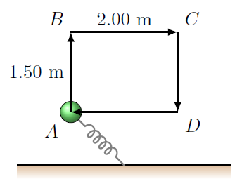
Fig. 20.2 A mass on a spring, moving in a rectangular path
Find the work done on the mass by the gravitational force as it completes one cycle around the rectangle.
Find the work done by the spring force along the path.
Find the work done by the force of air resistance. Assume that this force \({\vec F}_{AR}\) is given by \({\vec F}_{AR} = -C {\vec v}\), where \(C = 2.10\) kg/s.
Find the work that you do on the mass as you move it around the path. Hint: What is the net work done on the mass?
Answers: 0.00 J, 0.00 J, -25.0 J, 25.0 J
Problem
One of your shipmates goes to their laboratory and measures the work done by a force \({\vec F}\) between five points. They draw a graph of some of the results they obtained, as seen in the figure. The arrow indicate the direction for each displacement used; going against the arrow would give a work with the opposite sign. For example, the work done by the force when traveling from point \(A\) to point \(B\) is \(-4\) J, while traveling from point \(B\) to point \(A\), the work would be \(+4\) J. Is \({\vec F}\) a conservative force?
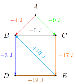
Fig. 20.3 The work done by a force \({\vec F}\) between marked points
Answer: You only need to check the simplest loops for this diagram; if these all meet the requirement of a conservative force, then so will other possible paths. However, you can see that there is a problem with edge \(BE\), since neither of loops \(BCE\) or \(BDE\) lead to zero around a closed path. For example, the total work done along the path \(B \to C \to E \to B\) is -6 J, not zero.
For conservative forces, the work \(W_F\) done by the force \({\vec F}\) is the same, regardless of which path you use to move from the starting to the final positions. This is why we can use the following definition for the potential energy of a generic conservative force \({\vec F}\), based on this work \(W_F\).
Quantity: potential energy
Symbol: \(U\)
Definition: The change in potential energy \(U_F\) for a conservative force \({\vec F}\) is defined in terms of the work \(W_F\) done by that work as
Units: joules (J)
Notice that the work done by the force only defines the change in potential energy. This means that only this change has physical consequences! Said a different way, the absolute size of the potential energy doesn’t matter, so we are free to choose a reference point \({\vec r}_{ref}\) where \(U_F (r_{ref}) = 0\). However, sometimes there is a natural choice of this reference point, either to make the calculations simpler, or there is a special point of physical relevance. This is something to keep in mind for the spring force (Hooke’s law), and the general form of gravitational potential energy (which we will see in Lesson 22).
20.3. Gravitational and spring potential energy
The first type of potential energy we will look at is that for the force of gravity. Remember in Lesson 19 that we showed the work done by gravity near the Earth’s surface is given by
Thus, we can see that this naturally fits into the pattern above, where the work done by a conservative force defines a change in potential energy. In other words, the work \(W_g\) depends only on the difference in vertical position \(r_y\), and not the path taken between this difference. We saw this earlier for the skater in the simulation earlier in the lesson; when there is no friction on the ramp, the skater always returned to the same height, where they had the same gravitational potential energy.
Quantity: gravitational potential energy
Symbol: \(U_g\)
Definition: Near the surface of the Earth (or any other large mass), the gravitational potential energy \(U_g\) is given by
where \(m\) is the mass of the object located at vertical position \(r_y\), and \(g\) is the magnitude of the gravitational field (9.81 m/s\(^2\)). Note: \(r_y = 0\) is the reference height where \(U_g = 0\) – you are free to choose this height!
Units: (kg)(m/s\(^2\))(m) = (kg\(\cdot\)m/s\(^2\))m = N \(\cdot\) m = J
Later on in Lesson 23, we will talk about the gravitational potential energy for a general position, not just near a large mass such as the Earth.
Problem
A child starting from rest slides down each of the four frictionless slides \(A\) to \(D\). Each has the same vertical height. Rank in order, from largest to smallest, her change in gravitational potential energy as she slides down each of the slides.
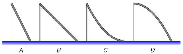
Fig. 20.4 Four possible slides
Answer: All four traverse the same vertical distance, so all four would give the child the same change in gravitational potential energy. The actual path does not matter, since gravity is a conservative force.
Problem
A penny (\(m\) = 2.50 g) is dropped from the top of the Empire State Building, which is 1250 ft tall. Assume that the gravitational potential energy is zero at the bottom of the building.
What is the gravitational potential energy (in J) of the penny at the top of the building?
What is the gravitational potential energy (in J) of the penny at the bottom of the building?
What is the change in the gravitational potential energy (in J) as the penny falls from the top of the Empire State Building to the ground?
How do your answers change if \(U_g = 0\) at the top of the building?
If \(U_g = 0\) at the midpoint of the building?
Answers: When \(U_g = 0\) at the bottom of the building, then \(U_g\) is +9.34 J, 0.00 J, and -9.34 J, for the top, bottom, and change in \(U_g\). When \(U_g = 0\) at the top, then the answers are 0.00 J, -9.34 J, and -9.34 J. Finally, when \(U_g = 0\) is chosen at the midpoint, then the answers are +4.67 J, -4.67 J, and -9.34 J. The changes in gravitational potential energy are the same for all three choices; the actual values at a particular point have no physical relevance.
The following clip looks at whether a penny dropped from the top of the Empire State Building can penetrate a person’s skull.
A second conservative force is the spring or elastic force \({\vec F}_{spr}\). Suppose a mass at position \({\vec r}\) is attached to a spring with spring constant \(k\) and equilibrium position \({\vec r}_0\). Then, from Lesson 23, the spring force is given by Hooke’s law, with
This was an example of a non-constant force, so to find the work done by the spring force, we needed to use the area under the curve. If you went through the vPython simulation and algebraic problems in Lesson 23, you would have seen that the work done by the spring force when the mass is moved from position \({\vec r}_i\) to \({\vec r}_f\) is
Again, this is the difference of two quantities, each of which depend only on the position of the object, either at the beginning or the end of its motion. The path taken between those two points does not matter. It also does not matter if the spring is compressed or stretched from its equilibrium position – moving it the same distance in either direction gives the same work, and therefore the same change in potential energy. Thus, the spring potential energy is given by
Quantity: spring (or elastic) potential energy
Symbol: \(U_s\)
Equation:
where \(k\) is the force constant or spring constant (units: N/m) and \(r\) is the distance a spring is compressed or stretched from the equilibrium position \({\vec r}_0\)
Units: (N / m)(m)\(^2\) = N \(\cdot\) m = J
Problem
The figures below show systems containing a block attached to the end of a spring resting on a frictionless surface. In each system, the springs are stretched or compressed by a distance given in the figure. The force constant and mass are also given for each system. Rank these systems on the basis of the elastic potential energy stored in the system.
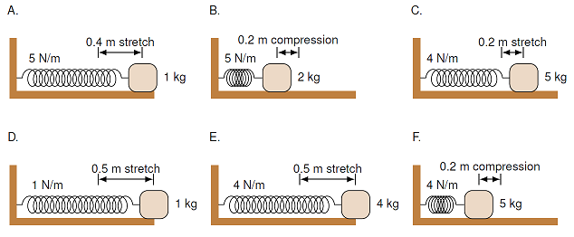
Fig. 20.5 Ranking the elastic potential energy of the systems
Answer: \(E > A > D > B > C = F\)
Problem
How much energy is stored in a spring that is stretched 3.00 cm as compared to the same spring if it were only stretched 1.00 cm? Choose the best answer below.
they have the same stored energy
three times
six times
nine times
twenty-seven times
Answer: When the spring stretched 3.00 cm, it has nine times the potential energy stored in it as when it is only stretched 1.00 cm.
Problem
A spring with a spring constant of 2400. N/m is initially compressed 10.0 cm from its equilibrium length. What is the change in elastic potential energy if you stretch the spring to 40.0 cm beyond its equilibrium length?
Answer: 180. J
20.4. Conservation of energy
We now have all the elements we need to talk about the conservation of mechanical energy. To do this, let’s start with the work-energy theorem from Lesson 19. For now, let’s just write kinetic energy as \(K\), so for a given system, the work-energy theorem says
Now, we can go through the list of all forces acting on the system, i.e. all forces included in the total work \(W_{tot}\). Some of these forces will be conservative forces, and thus have their own potential energy; the rest of these forces will be non-conservative. Therefore, we can write the total work as the sum \(W_c\) of the work done by conservative forces, and the sum \(W_{nc}\) of work done by the non-conservative forces.
The work \(W_c\) is made up of the changes in potential energy for all the conservative forces. Thus, if we have conservative forces \({\vec F}_1, {\vec F}_2, \cdots\), up through \({\vec F}_j\), for an index \(j\), then each will do a work \(W_j = -\Delta U_j\). So the sum is
But this sum of the differences is the same as the difference in the sums!
Let’s write these in terms of summations, as a way to put these equations together:
In the last step, we have added together all of the initial potential energies of the system and called it \(U_i\); similarly, \(U_f\) is the sum of all the final potential energies of the system. Putting this back into the work-energy theorem,
Moving the change in total potential energy to the right-hand side gives
Thus, when there are no non-conservative forces (i.e. \(W_{nc} = 0\)), the sum of all the kinetic and potential energies of the system remains the same. This is an important result, so we give this sum the name mechanical energy \(E\).
Quantity: mechanical energy
Symbol: \(E\)
Definition: Mechanical energy \(E\) is defined as the sum of all kinetic and potential energies for a system:
Units: J
In practice, this means adding in all possible forms of these energies; at this moment, mechanical energy includes gravitational and elastic potential energies:
The general statement of conservation of energy relates the change in the mechanical energy to the work done by non-conservative forces
In the absence of non-conservative forces (friction, air resistance), mechanical energy is conserved:
or
This last equation will be our typical starting point. It is good practice to begin with the most general case, and think about which kinds of energy are present at the initial and final states of the system. Choosing these states cleverly will help greatly as well!
It may helpful to look at particular situations, so you can see how the changing state of a system relates to the kinetic, potential, and mechanical energies. If you go back to the simulation of the skater previously mentioned in this lesson, you can see how the kinetic and gravitational potential energies of the skater depending on the ramp shape and height. Use the pie chart or bar graph for pictorial representations of the various energies as the skater moves along the ramp.
Here is another related simulation, where the motion of a mass on a vertical spring can be studied. Select “Energy” when the app loads up, so you make look at the various types of energy in the system.
20.5. An example: A block on a spring
Let’s go through an example, and see how the conservation of mechanical energy works. Suppose a 150. g wooden block is placed on top of a vertical spring, and it comes to rest at a distance of 2.64 cm from the spring’s equilibrium point. The block is pushed down a further 5.36 cm, and then released. We are going to find the maximum height the block will momentarily reach over the equilibrium position of the spring.
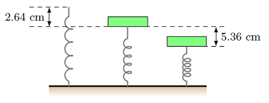
Fig. 20.6 Vertical spring with a block set on it
The first thing to realize is that in the middle position, where the block is at rest on the vertical spring, is not where the “energies balance out”. The block is at rest because the net force at this location is zero; if this was not true, the spring and block would start accelerating. Thus, we first need to use Newton’s second law here. This will allow us to calculate the spring constant of the vertical spring, which we do not know at this point. The net force on the block is due to the upward force \(F_{spr}\) on the block from the spring, as well as the downward force \(F_g\) of gravity. Setting the magnitudes of these two forces equal to each other,
then the spring constant \(k\) is equal to \(k = mg / \Delta r_y\). Here, \(\Delta r_y\) is the vertical distance from the equilibrium point of the spring to where the block comes to rest, and so \(\Delta r_y = 2.64\) cm (as a magnitude, since we have already taken into account the signs in the equation above).
Now we can look at what happens when the block is pushed down further. The net force will not be zero here, since the spring force is larger than the block’s weight. This is why the block will accelerate upward until it is pushed completely off the spring. Since the spring force depends on the distance the spring is away from its equilibrium, we cannot use the kinematic equations – the acceleration changes with time, so it is not constant! This is why using the conservation of mechanical energy is the best choice: we only need to know what is happening between the initial state (when the block is pushed down to its lowest point) and the final state (the block has left the spring, so the spring is no longer compressed).
So, we start with \(W_{nc} = 0\) (no friction), and write down the conservation of mechanical energy equation,
If we take the initial and final states outlined in the paragraph above, then the block is (momentarily) at rest at both of these points. This means \(K_i = K_f = 0\). The spring is also not compressed in the final state, since the block is no longer sitting on it, giving \(U_{s, f} = 0\). The block is compressing the spring at the beginning, however, so \(U_{s, i} \neq 0\) from the total compression \(r\) of \(2.64 + 5.36 = 8.00\) cm from the equilibrium. Last, we turn to the gravitational potential energy. Here we need to make a choice about where to put the reference height. This is different than the choice for the spring potential energy, which was already chosen (when \(U_s\) was defined) to be the spring’s equilibrium position. Since there is no strong reason to choose one height over another, let’s pick the block’s final position as the height where \(U_g = 0\). This gives \(U_{g, f} = 0\) and \(U_{g, i} = mgh\), where \(h < 0\) is the distance from the starting and ending heights of the block – negative since the initial position is below the final. Thus, our final energy conservation equation is
We can solve for \(h\) to get
In the last step, we used the equation for the spring constant \(k\) we got earlier when the net force was zero. Note that the mass of the block doesn’t matter! Plugging in the numbers, and taking the absolute value, we have \(|h| = 12.12\) cm. However, this is the total distance from the initial to the final heights, and we want only the height above the spring’s equilibrium point. So, we subtract 8.00 cm from 12.12 cm to get 4.12 cm for our final answer.
Problem
A block of mass \(m = 2.50\) kg situated on a smooth incline at an angle of \(\theta = 37.0^\circ\) is connected to a spring of negligible mass. The pulley is frictionless. The block is released from rest when the spring is unstretched. The block moves 13.0 cm down the incline before coming to rest. Find the force constant (in N/m) of the spring.
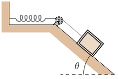
Fig. 20.7 Block on a ramp and attached to a horizontal spring
Answer: 227 N/m
Problem
A 5.70 kg block starts on a ramp above a frictionless surface. At the opposite end of the flat surface is a spring, with a spring constant of 670 N/m. The figure is drawn to scale, with each grid square having sides of 25.0 cm. After letting go of the block on the ramp, it moves across the surface to hit the spring. Calculate the position (in cm) where the spring momentarily stops the block.
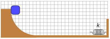
Fig. 20.8 A mass slides down a ramp and is stopped by a spring
Answer: 50.0 cm from the spring’s equilibrium point
20.6. Non-conservative forces and mechanical energy
In the situations given above, we did not include any non-conservative forces. Remember that these would be forces such as friction or air resistance, and would change the mechanical energy of the system. This is the natural next step for extending our energy methods. If an object encounters a non-conservative force between its initial and final states, then \(W_{nc} \ne 0\) – mechanical energy is added to, or removed from, the system and \(\Delta E \neq 0\). Note that this equation can be written as
The right-hand equation tells the story: the system starts with a mechanical energy \(E_i\), then in the process of going from the initial to the final state, there is an energy flow (or work) \(W_{nc}\), leading to a final mechanical energy \(E_f\). Another way to write this matches what was done above, where the initial mechanical energy is now on the left, as is the non-conservative work \(W_{nc}\):
Here are some practice problems to give this modified energy equation a whirl. Remember that these problems just combine what we have done in this lesson and the last – for the non-conservative forces, you have to find the work by those forces using the methods of Lesson 23; otherwise, it is an energy problem as we have done in this lesson.
Problem
In the figure below, a block of mass \(m = 2.00\) kg is compressing a spring a distance \(d = 6.00\) cm when it is released. The block travels over a rough spot, after which it has a speed of \(v = 1.00\) m/s. The rough spot has a length of 7.50 cm and \(\mu_k = 0.200\). What was the spring constant of the spring?
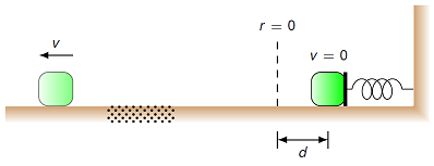
Fig. 20.9 Block launched by spring, and passes over a rough spot
Answer: 719 N/m
Problem
A 5.70 kg block starts on a ramp above a frictionless surface. At the opposite end of the flat surface is a spring, with a spring constant of 670 N/m. The figure is drawn to scale, with each grid square having sides of 25 cm. After letting go of the block on the ramp, it moves across the surface to hit the spring. There is a rough patch along the way of distance \(d\), with a coefficient of kinetic friction \(\mu_k = 0.375\). Calculate the position (in cm) where the spring momentarily stops the block.
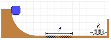
Fig. 20.10 A mass slides down a ramp passes over a rough patch before being stopped by a spring
Answer: 36.5 cm form the equilibrium point
20.7. Energy graphs
Let’s go back to a situation like we had earlier, with the vertical spring example. Suppose we have an ideal spring again, with spring constant \(k\), placed so that it is aligned vertically. The spring will have some equilibrium length \(r_{0, y}\). Since the spring is ideal, it has no mass of its own, but we can imagine placing a block of some mass \(m\) on top of the spring. The spring-mass system will have both gravitational and spring potential energy; thus, the total potential energy \(U\) of this system is
where \(r_y\) is the vertical position component of the mass. If we graph this function, we get the plot shown below.
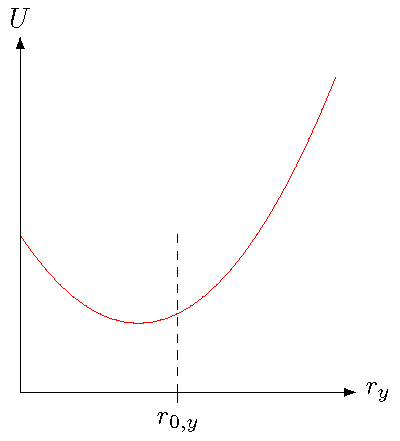
Fig. 20.11 Total potential energy of the spring-mass system
In the graph, I have marked the equilibrium position \(r_{0, y}\) of just the spring. However, the value of \(U\) is not lowest at that point, because of the addition of the gravitational force, and its contribution to the potential energy. The point where the potential energy is lowest is the equilibrium point when both the spring and gravitational forces on the mass are taken into account! Remember in the vertical spring example above, the mass was placed on the spring, and came to rest at a distance of 2.64 cm below the equilibrium of the spring. This would be the point where the total potential energy is the least. I will come back to that point in a bit.
Now, let’s imagine that we place the mass on the spring, and press it down some further distance. Before we let go of the mass, all of the system’s energy will still be potential energy – no motion, no kinetic energy. I have placed a point \(r_{bot}\) on the graph below to show this bottom point. I will explain the rest of the graph as we go along.
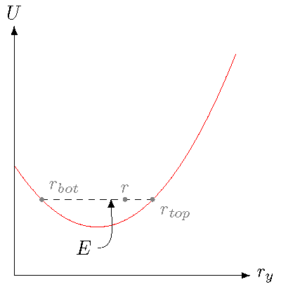
Fig. 20.12 Motion of the spring-mass system, using the potential energy graph
So, what will the system do after I get go? Hopefully, you are not surprised that the mass starts moving upward. I will describe this in two different ways. First, let’s talk about it in terms of the separate forces of gravity and the spring. Since the mass is now below the equilibrium point it was resting at before, the spring force has a larger magnitude than the gravitational force, and the mass is pushed upwards. This is because the spring has an even greater compression than it did when the mass was motionless, which increases the size of the spring force.
However, there is a second way to predict the motion, based solely on the graph. Intuitively, imagine the point \(r_{bot}\) as if there was a ball placed on the graph. You would expect the ball to “roll downhill”, to the right of the graph. This intuition matches a more rigorous description. Since both the gravitational and spring forces are conservative, we can say the total potential energy \(U\) graphed above is related to the total force \({\vec F}_{net}\) by
Let’s use the fact that the displacement \(\Delta {\vec r}\) is only vertical, so \(\Delta {\vec r} = (\Delta r_y) {\hat y}\). This gives that the magnitude \(F_{net}\) of the net force is related to the change \(\Delta U\) in potential energy by
If I rearrange this, we get
This is just the (negative of the) slope of the graph! Since the slope of the \(U\) vs. \(r_y\) graph is negative at \(r_{bot}\), then the force is positive, i.e. to the right, which means the mass will move to higher \(r_y\).
Force is slope of potential energy vs. position
Suppose an object moves along a line, with position \(r\), due to the influence of a potential energy \(U(r)\). The net force \({\vec F}\) on the object will be
Now we can see why the equilibrium point for the system is at the point when the potential energy \(U\) is at its smallest. At that position \(r_y\), the slope of the graph is zero, so the net force on the object will be zero there as well. Again, think of the analogy of the ball; if you place a ball at that point, it will not start rolling uphill! This equilibrium point is known as a stable equilibrium: a position where the net force is zero, and where moving a small distance to either side means the system experiences a net force which returns it back to the original point. This is opposed to an unstable equilibrium, where the force is zero precisely at the point, but moving just a little bit away gives rise to a net force that amplifies that motion. Think about balancing a pencil on its point; you can do it if you are careful, but the slightest motion will make the pencil fall down.
Let’s now get back to the graph. Notice that I have drawn a dashed horizontal line on the graph; this line is placed at the value of the mechanical energy \(E\) for the mass. Obviously, this touches the \(U\) curve at the point \(r_{bot}\), since the mass is motionless there, so the kinetic energy \(K = 0\). But why did I draw this line? Because it tells us what the motion of the mass will look like after we let go of it. Again, as we saw above, when the mass is at \(r_{bot}\), the force on it is in the \(+y\) direction, so the mass will move upward. On the potential energy graph, as you move to the right, there is a gap between the dashed line for \(E\), and the potential energy \(U\). What is this gap? It is the difference \(E - U\), which is precisely the kinetic energy \(K\) of the system! Thus, just from the graph, we can see that the mass will initially speed up with increasing \(r_y\). However, once the mass passes the equilibrium point for the system, the gap gets smaller, and the mass will slow down. Eventually, the mechanical energy \(E\) of the system will equal the potential energy \(U\) at the vertical distance \(r_{top}\). At this point, the mass will stop, and then start moving downward. Because there are no non-conservative forces, this motion will repeat indefinitely, with the mass oscillating between the highest and lowest points \(r_{top}\) and \(r_{bot}\), respectively.
Problem
The graph show the potential energy \(U(r_x)\) of a 65.0 g object moving under the influence of an outside conservative force. At \(r_x = 0.00\) m, the object is moving in the positive \(x\) direction at 2.89 m/s.
What is the mechanical energy (in mJ) of the object?
What is the net force on the object at \(r_x = 2.50\) m? Give the vector in unit vector notation, in mN.
What is the speed (in m/s) of the object when it reaches \(r_x = 4.00\) m?
What is its speed (in m/s) when it reaches \(r_x = 7.00\) m?
Suppose the starting speed of the object was 2.25 m/s. Does it reach the point \(r_x = 8.00\) m? If not, where does it stop?
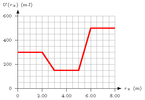
Fig. 20.13 Potential energy vs. position graph
Answers: 571 mJ; \((+150. \textrm{ mN}) {\hat x}\); 3.60 m/s; 1.48 m/s; the block stops at 5.90 m
20.8. The effective potential energy
20.8.1. Constant central force
The discussion above was only for motion along a single dimension, such as the \(y\) axis for the vertical spring. However, we are heading towards considering planets orbiting around a star when we get to Kepler’s laws in Lesson 23. You might think adding a spatial dimension would make the graphs more complicated (since they would now be three dimensional!). In general, this is the case, but it turns out things remain relatively simple if we consider only central forces, which we talked about in Lesson 16 and Lesson 18. Remember that a central force is a force vector only pointing along the radial vector \({\vec r}\), i.e. a force which generates zero torque around the \({\vec r} = {\vec 0}\) point.
To start with, let’s return to the central force \({\vec F}_c\) with constant magnitude we used as an example in those earlier lessons. Since the magnitude is constant, then we can easily find its potential energy function \(U_F\). In fact, this will be very similar to what we did with the gravitational potential energy \(U_g\) previously in this lesson, from a constant gravitational field \({\vec g}\). The only difference is that the central force points in the radial direction \({\hat r}\), so its potential energy is
Thus, we can write down the mechanical energy \(E\) of the object as the sum of its kinetic and potential energies. However, before I do this, I will use the Pythagorean theorem to decompose the velocity into its radial and perpendicular components \(v_r\) and \(v_\perp\), respectively. After this step, I have the mechanical energy is
Suppose we want to know what the inner and outer radii are of the orbit. In other words, what is the smallest distance \(r\) the object gets to the center \({\vec r} = {\vec 0}\)? What is the largest distance it gets from the center? Since we only care about the radial motion of the object, let’s do something clever. I will group together everything that is not the kinetic energy piece depending on \(v_r\) into a single part \(U_{eff}\), with
This is known as the effective potential energy, defined as
Using \(U_{eff}\) allows us to focus purely on the radial motion of the system; we can treat the object as moving only in \(r\) due to the effective potential energy of the system.
In particular, we can find the velocity component \(v_\perp\), at a given radius \(r\), once we know the constant magnitude \(L\) of the angular momentum of the system. Remember in Lesson 18 that we can write the magnitude \(L\) of the angular momentum for a point mass in terms of the perpendicular velocity component \(v_\perp\) as
With some algebra, you can show that
This is a step forward, since the magnitude \(L\) is constant for central forces; therefore, this term is now only a function of the radial distance \(r\). This means that now the effective potential \(U_{eff}\) is also just a function of \(r\). So we can analyze the system by looking only at how the object changes its radius over the course of its motion, ignoring the perpendicular piece entirely.
I show this by using the central force simulation we saw previously in Lesson 18 for the constant central force. In this version, I have put in an energy graph with two curves: the effective potential \(U_{eff}\) in blue, and the mechanical energy \(E\) in green. Since mechanical energy is conserved, the green line is flat; the difference between the green and blue curves is the radial piece of the kinetic energy, i.e. the part that depends on \(v_r\).
Notice that we now have another way to explain why the ball never goes closer to the center than some fixed radius. Remember, when I first introduced this central force in Lesson 16, I described this inner radius in terms of the constant central force \({\vec F}_c\) versus the necessary centripetal force to keep it in circular motion. There, for radii \(r\) when \(F_c - mv^2 /r < 0\), the net acceleration is not enough to keep it moving in a circle, so the radial velocity component \(v_r\) will slow down, until the object stops moving inward at the inner radius, and starts moving outward. Using what we have talked about in this lesson, we can express this same process, but in terms of energy. As the ball approaches the inner radius, an increasing amount of its mechanical energy \(E\) is in the perpendicular piece \(L^2 / 2mr^2\) of the kinetic energy, while the radial part \((1/2) mv^2 _r\) will decrease in size. Eventually, there is no available energy for the radial portion, so \(v_r = 0\), and the ball turns around. The turning points of the ball (both inner and outer) are when the mechanical energy \(E\) equals the effective potential energy \(U_{eff}\). There is an “energy barrier” to the ball moving too close to the center, due to its angular momentum!
Thus, we now have enough information to solve for these turning points of the ball – those radial distances \(r\) where the ball is at its maximum and minimum distance from the center. To do this, let’s first find the mechanical energy \(E\) of the system, using the initial values in the program. With \(F_c = 10\) N/m, \(m = 4\) kg, \(r = 5\) m, and \(v = 3\) m/s, then
Now, at the turning points, this mechanical energy will equal the effective potential energy, with
In other words, the object has momentarily stopped its radial motion, so there is no radial kinetic energy at the turning point. Recall from when we went through this simulation previously in Lesson 18 that the magnitude \(L\) of the angular momentum was 60.0 kg m\(^2\) / s\(^2\). Thus, with a little bit of algebra, this last equation becomes an equation for the unknown \(r\), with
This may look daunting, since it is a cubic equation. However, if you try the starting radius \(r = 5\), you will see that this gives a solution to the equation – the ball begins at one of its turning points. It turns out that knowing this root is enough to solve for the other roots. Let’s plug in the numbers, so it is more obvious what is going on. This gives (dropping the units)
However, since \(r = 5\) is a root, then \((r - 5)\) is a factor of this polynomial, so that
for some unknown coefficients \(a, b, c\). Thus, when \(r \ne 5\), it is the second factor that must be zero; this can be easily solved for the last two roots of the polynomial. The two positive solutions of the overall equation will be the outer and inner radii of the object’s motion.
Problem
Solve for the unknown coefficients \(a, b, c\) in the second factor, then use the quadratic formula to get the radius of the other turning point.
Answers: \(a = 10, b = -18, c = -90\); the other positive solution is \(r = 4.03\) m.
Problem
Use conservation of angular momentum to find the speed of the object when it reaches its outermost turning point. Do you get the same answer if you use conservation of energy instead?
Answer: 3.72 m/s
20.8.2. The spring force
Everything I said above for the constant central force also applies to any other central force. Thus, given a central force, an object moving solely due to this force will have an effective potential energy. We can then explore the properties of the motion with other central forces using the same techniques. To see this, below is a modified version of the mass on a spring program we saw in Lesson 19. I have added an effective potential energy graph, much like what I did earlier, and the mass is given an initial velocity \({\vec v}\) that is perpendicular to its position vector \({\vec r}\). Run the program, and notice how the motion matches the effective potential energy graph.
As we saw earlier in this lesson, the spring potential energy is given by
This means that the effective potential energy for a mass on a spring is now
You can go through the same analysis as we did above to find the turning points of the mass-spring system; do this in the next problem.
Problem
Use the default values of the appropriate variables in the mass on a spring program above (assigning them the proper SI units) to answer the following questions. You can compare your calculated answers to those shown in the graph after you run the program.
What is the mechanical energy of the system (in J)?
What is the magnitude of the mass’ angular momentum (in kg m\(^2\)/s\(^2\))?
What are the two turning points (in m) for the mass? Hint: If you use the process described earlier, you will get a quadratic equation in the variable \(r^2\) (not \(r\)). Solve this equation for the values of \(r^2\), then find the positive solutions for \(r\).
What is the speed of the ball at its innermost radius?
Suppose you change the initial speed so that it is now 2.50 m/s; do not change any of the other variables. What would be the turning points of the mass in this scenario? Note the angular momentum magnitude is now different!
Answers: 14.6 J; 22.5 kg m\(^2\)/s\(^2\); 2.37 m and 3.00 m; 1.90 m/s; 3.00 m and 3.95 m
Now, suppose the initial velocity is not perpendicular to the radial position vector \({\vec r}\). Let’s change initial velocity in the program above, so it has the same magnitude, but a different direction. Change the code
INIT_SPEED = 1.5 # Initial speed (m/s)
so it now reads
Q = 30                    # Initial velocity angle
INIT_VEL = 1.5 * vector(cos(radians(Q)), sin(radians(Q)), 0)
Inside the definition of ball, you will need to assign the attribute ball.velocity to be INIT_VEL. The initial velocity now points at a \(\theta = 30.0^\circ\) angle to the \(+x\) axis, rather than strictly along the \(+y\) axis, as before. This change means that the initial velocity has both a perpendicular component and a radial component at the start. Because of this, the motion will be different; if you run the program, you will see the ball moves further out, along a “tilted” ellipse. The change in the initial velocity means the angular momentum magnitude has changed; we can solve for its new value (using the original speed \(v\) of 1.50 m/s) by
Plugging in the default values, along with the new angle \(\theta\), gives \(L = 11.3\) kg m\(^2\)/s\(^2\). The new angular momentum magnitude has changed the shape of the effective potential energy, which is noticeably more asymmetric in the radial direction. However, the mechanical energy \(E\) has not changed, since the initial speed is exactly the same as before! We can use these numbers to solve for the turning point radii as we did previously.
Problem
Start the mass on the spring with an initial speed of 1.50 m/s, at an angle \(\theta = 30.0^\circ\) from the \(+x\) axis. Calculate the turning point radii of the ball (in m). Verify your answers by running the modified program above.
Answers: 0.961 m and 3.70 m
Problem
In this new situation, find the speed of the mass at its new turning points.
Answers: At the inner turning radius, the mass is moving at 2.34 m/s; at its outer turning point, its speed is 0.608 m/s.
20.8.3. Finding the stable equilibrium
For both the constant central force, and the spring force, you may have noticed that both graphs look basically the same (although not exactly!). In particular, both are “bowl shaped”, so there is a radius in each case where the slope of the effective potential is zero. Much like we talked about in the last section, this radial distance would be where the object is at a stable equilibrium; if the object were placed slightly away from this point, they would oscillate around the equilibrium distance.
It is important to note what is being said here. When I talk about just the potential energy, like I did in the last section, I am considering only motion along a single direction – imagine the mass on a spring moving back and forth on the \(x\) axis. Then, the stable equilibrium point is where the mass would be completely stationary. However, when I talk about the effective potential energy, I am talking about two dimensional motion, since \(U_{eff}\) includes the angular momentum of the object moving perpendicular to the radial direction. Here, the stable equilibrium would be that radius \(r\) and perpendicular velocity component \(v_\perp\) such that the radius does not change. In other words, the object is moving in a circular orbit at precisely this equilibrium distance \(r\).
To flesh this out, let’s go back to the constant central force \({\vec F}_c\) and find the stable equilibrium radius for the angular momentum \(L\) for the default values. We have to keep \(L\) the same as the original value, or else the effective potential energy graph would change! Thus, we want to solve the following equations for the equilibrium radius \(r_e\) and the perpendicular velocity component \(v_\perp\):
The first is just the fact we are keeping the angular momentum magnitude the same, so that the effective potential energy graph is the same; the second is Newton’s 2nd law, relating the constant force magnitude \(F_c\) to the net force. You can solve these algebraically for either \(r_e\) or \(v_\perp\) in one equation, then subtitute into the other equation, to get equations for \(r_e\) and \(v_\perp\). For the equilibrium radius \(r_e\) in particular, this gives
With the default values in the program, and the angular momentum magnitude \(L = 60.0\) kg m\(^2\)/s\(^2\) we found previously, then the equilibrium radius \(r_e = 4.48\) m. You can run the earlier program to verify this is the bottom of the effective potential graph.
Problem
Use the default values of the appropriate variables in the mass-spring program above, and find the equilibrium radius \(r_e\) for the mass on a spring. Note you will get a different algebraic equation for \(r_e\), since the force is different. Run the program and verify your answer using the effective potential energy graph.
Answer: 2.67 m
20.9. Summary
Energy methods are one of the most powerful techniques in physics. Notice that it is all in one equation! That is one of the advantages of using conservation of energy. In fact, if you decide to pursue physics as a major, you will see that many of the more advanced methods you will see are just different versions of writing down the mechanical energy of the system.
The flip slide, though, is that all the energies are scalars, so information about direction is lost. For example, you can use mechanical energy to find the speed of an object at a given position, but not its velocity, since you cannot determine the drection using a scalar. However, with that being said, you can learn a lot from using the conservation of mechanical energy.
After this lesson, you should be able to:
Define mechanical energy.
State the principle of conservation of mechanical energy.
Use the change in mechanical energy equation to solve for an unknown quantity such as the speed or position of an object at a particular time.
State the relationship between a conservative force, and the slope of the force’s potential energy vs. position graph.
Define the effective potential energy of a system.