.ipynb .pdf

Binder

Contents

11. Center of mass and collisions

11.1. Overview

So far, I have been avoiding a key part of physics. Over all of the lessons so far, we have talked about how and why objects move. Specifically, given the acceleration of an object, we can find its position and velocity; with Newton’s laws, we can start to calculate acceleration ourselves! But what is doing the moving? In particular, when I say the position of an object has changed, what point of the object has shifted? We have glossed over this part, but it is actually important to consider.

It turns out that for motion in a line, instead of thinking of a given object as an extended mass – that is, with some finite shape and size – I can think of its mass as concentrated at a specific point. This point is called the “center of mass”. All of the physics we have done so far is then describing the motion of this point because of interactions with other objects. Hopefully, this is an obvious statement, but it is something that has to be proven. In fact, this need for a proof is one of the reasons Newton developed calculus!

Note that I was careful to say “motion in a line”. When rotation gets involved, then the shape and size of the object become important again. We will ignore those complications. This lesson will introduce the concept of the center of mass, and how it applies to collisions in one dimension.

Here are the objectives for this lesson:

• Define the center of mass position and velocity of a group of objects.

• Describe how Newton’s 3rd law is equivalent to conservation of momentum for an isolated system.

• Calculate the unknown mass or velocity of an object experiencing a collision in one dimension using conservation of momentum.

• Define the coefficient of restitution.

• Define elastic and inelastic collisions in terms of the coefficient of restitution.

11.2. Center of mass

When you calculate your grade in this class, you know that you weigh different types of grades differently – tests count more than homeworks, for example. Your grade is a “weighted average” of what you earn on various assessments. In the same vein, the “center of mass” (or CM) is also a weighted average, but now over the mass in an object. If we consider the CM to be a specific point associated with an object, or system of objects, then we can define various quantities describing that point and its motion. Thus, we start with the position of this CM point.

Center of mass position

The center of mass position \({\vec r}_{CM}\) for a group of objects is defined as the average of the positions, weighted by the mass of each object, or

\[ {\vec r}_{CM} = \frac{\sum_i m_i {\vec r}_i}{\sum_i m_i} = \frac{m_1 {\vec r}_1 + m_2 {\vec r}_2 + \cdots}{m_1 + m_2 + \cdots} \]

The video below does a good job of demonstrating this idea of the CM and its motion.

If you think about it, the CM will be closer to the points where there is more mass, and further away from the places where there is less. This is what it means to have a “weighted average”. Note that the SI units for \({\vec r}_{CM}\) are still meters, since the mass units cancel out in the ratio.

Problem

Find the center of mass position (in cm) of the following mass distribution. The origin is at the center of the rectangle. Give your answer in unit vector notation.

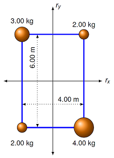
Fig. 11.1 Find the center of mass of the four objects in the picture

Answer: \({\vec r}_{CM} = (18.2 \textrm{ cm}) {\hat x} + (-27.3 \textrm{ cm}) {\hat y}\)

Problem

A uniform piece of thin sheet metal is shaped as shown below. Calculate the position (in cm) of the center of mass, and give your answer in unit vector notation.

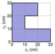
Fig. 11.2 Find the CM position of an extended object

Answer: \({\vec r}_{CM} = (11.7 \textrm{ cm}) {\hat x} + (13.3 \textrm{ cm}) {\hat y}\)

Let’s learn how to use physics to be a better athlete! One famous use of the idea of center of mass is the “Fosbury flop”, a new technique for the high jump that allowed competitors to raise the bar higher than it ever had been before. This is featured in the video.

Similar to how the CM position was defined, for a system of moving objects, we also have the center of mass velocity.

Center of mass velocity

The center of mass velocity \({\vec v}_{CM}\) is defined as a weighted average of all the individual velocities:

\[ {\vec v}_{CM} = \frac{\sum_i m_i {\vec v}_i}{\sum_i m_i} = \frac{m_1 {\vec v}_1 + m_2 {\vec v}_2 + \cdots}{m_1 + m_2 + \cdots} \]

Notice that, using the idea of momentum \({\vec p}\), then the total momentum \({\vec P}\) of the system of objects can be expressed as

\[ {\vec P} = \sum_i {\vec p}_i = \sum_i m_i {\vec v}_i = M {\vec v}_{CM} \]

where \(M\) is the total mass of the objects

\[ M = \sum_i m_i = m_1 + m_2 + \cdots \]

When we talked about the motion of a system in Lesson 10, this was referring to the velocity of the system CM. The system is considered to be located at its CM position. Notice the special symbol used for the sled and truck system’s CM position on the right-hand side of the diagram below; you may see it again in an engineering course.

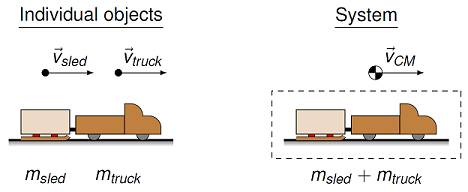
Fig. 11.3 The center of mass of a system of objects

Problem

Suppose the masses \(m_A = 4.55\) kg, \(m_B = 6.19\) kg and \(m_C = 2.83\) kg, shown below, are moving with the given velocities. Give your answers in unit vector notation.

1. What is the center of mass position (in m) of the system at the instant shown?

2. What is the center of mass velocity of the system (in cm/s)?

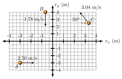
Fig. 11.4 Find the CM position and velocity of the moving objects

Answers: \({\vec r}_{CM} = (-0.615 \textrm{ m}) {\hat x} + (1.34 \textrm{ m}) {\hat y}\); \({\vec v}_{CM} = (43.1 \textrm{ cm/s}) {\hat x} + (-32.6 \textrm{ cm/s}) {\hat y}\)

Challenge

Suppose you have a stack of identical blocks, with a length \(L\). If you are careful, you can balance the stack on the edge of a table, so that the top block overhangs the table edge by some distance \(d\). What is the maximum distance \(d\) for two blocks, in terms of the length \(L\)? For three blocks? What is the minimum number of blocks needed for the overhang \(d\) to be greater than the length \(L\)? To be twice as much? Write a Python program that calculates the ratio \(d / L\) for a given number of blocks.

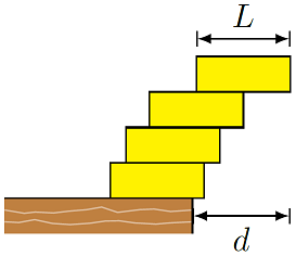
Fig. 11.5 Stacking blocks on the edge of a table

11.3. Collisions

11.3.1. The momentum of an isolated system

Suppose a system is made of two objects \(A\) and \(B\). The sum of the forces on the system is given by

\[ \sum {\vec F}_{sys} = \sum {\vec F}_A + \sum {\vec F}_B \]

If we use Newton’s 2nd law, this is the same as

\[ \sum {\vec F}_{sys} = \frac{\Delta {\vec p}_A}{\Delta t} + \frac{\Delta {\vec p}_B}{\Delta t} = \frac{\Delta ({\vec p}_A + {\vec p}_B)}{\Delta t} = \frac{\Delta {\vec P}}{\Delta t} \]

where \({\vec P}\) is the combined momentum of the system.

In order to simplify the physics of a situation, it is frequently helpful to consider a group of objects where the primary forces are between the objects. In other words, the net force on each object in the group is all due to interactions with other objects in the group; the external forces on the system add up to the zero vector. This is known as an isolated system. Collisions and explosions are a good example of this, since the outside forces (e.g. friction) have little effect compared to the forces between the objects in the system.

Remember that in Lesson 10, it was shown that the net force on a system is the sum of the external forces acting on the system (using Newton’s 3rd law).

\[ \sum {\vec F}_{sys} = \sum {\vec F}_{sys, out} \]

We just showed that the net force on the system is also equal to the change in the total momentum of the system, or

\[ \sum {\vec F}_{sys} = \frac{\Delta {\vec P}}{\Delta t} \]

If the system is isolated, then \(\sum {\vec F}_{sys, out} = {\vec 0}\), which means that the total momentum of the system does not change:

\[ \sum {\vec F}_{sys} = \sum {\vec F}_{sys, out} = {\vec 0} \Rightarrow \frac{\Delta {\vec P}}{\Delta t} = {\vec 0} \]

This is known as the conservation of linear momentum, and is one of the bedrock ideas of physics! Whenever we can say that some quantity stays the same (or is “conserved”) in a physical interaction, this allows us to describe the motion in much better detail.

Conservation of linear momentum

The total linear momentum of an isolated system stays constant.

Thus, if we add up the initial momenta of all the objects in an isolated system, this will be the same as the sum of the final momenta:

\[ \sum {\vec p}_i = \sum {\vec p}_f \]

Above, we showed that the total momentum of a system is equal to the total mass of the system multiplied by the center of mass velocity. With total mass \(M\), this means

\[ \sum {\vec F}_{sys} = M \biggl( \frac{\Delta {\vec v}_{CM}}{\Delta t} \biggr) \]

Thus, another way of saying that momentum is conserved is that the CM velocity of an isolated system is constant:

\[ M \biggl( \frac{\Delta {\vec v}_{CM}}{\Delta t} \biggr) = {\vec 0} \]

This leads to an important idea: for a system of constant mass, a constant total momentum is the same as a constant center of mass velocity. Remember that from Newton’s 2nd law, the force acting on an object will change its momentum. So another way to say the above is

No forces, no CM acceleration

An isolated system will have a constant center of mass velocity.

Let’s now see how this works in calculations. For the following two problems, use the conservation of momentum for the system to solve for the unknown velocity. The balls are only moving in one dimension, so there is only one vector component equation to worry about, but you have to use conservation for the system, meaning both masses are included in that equation.

Problem

A 2.00 kg red bowling ball, moving to the right at a speed of 3.00 m/s on a frictionless table, collides head-on with a stationary 2.50 kg green bowling ball. The green ball leaves the collision at 2.67 m/s to the right.

1. What is the velocity of the red ball (magnitude in cm/s) afterwards?

2. If the collision happens in 75.0 ms, what is the force on the red ball (magnitude in N) due to the green ball?

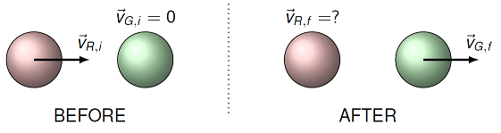
Fig. 11.6 A red ball strikes a stationary green ball

Answers: 33.8 cm/s, to the left; 89.0 N, to the left

Problem

Suppose we start the same way as the previous problem – a 2.00 kg red bowling ball, moving to the right at a speed of 3.00 m/s on a frictionless table, collides head-on with a stationary 2.50 kg green bowling ball – but now the green ball leaves the collision at 2.00 m/s to the right.

1. What is the velocity of the red ball (magnitude in cm/s) afterwards?

2. If the collision happens in 75.0 ms, what is the force on the red ball (magnitude in N) due to the green ball?

Answers: 50.0 cm/s, to the right; 66.7 N, to the left

11.3.2. Coefficient of restitution

The collision between the two objects will change their velocities. In the last two problems of the previous section, the two collisions started with the same information, but had different final velocities. What was the difference? One way of saying it is that the interaction force between the two bowling balls was different – the second collision was “less springy”, so the force between the balls was smaller. However, this force depends on the masses of the objects. Can we characterize the collision only by the velocities? This leads to the idea of the elasticity of the collision, which can be given by the coefficient of restitution. The coefficient of restitution is given the symbol \(\epsilon\) (the Greek letter “epsilon”). It can depend on the shape of the colliding objects, their speeds and composition.

• Quantity: coefficient of restitution

• Symbol: \(\epsilon\)

• Definition: The ratio of the final to initial relative speeds. For two colliding objects 1 and 2, with initial velocities \({\vec v}_{1i}, {\vec v}_{2i}\), and final velocities \({\vec v}_{1f}, {\vec v}_{2f}\), the coefficient of restitution is

\[ \epsilon = \frac{|{\vec v}_{1f} - {\vec v}_{2f}|}{|{\vec v}_{1i} - {\vec v}_{2i}|} \]

• SI units: unitless

Notice that this is a ratio of vector magnitudes, indicated by the absolute value signs.

The collision can be classified by the value of \(\epsilon\).

1. If \(\epsilon = 1\), the two objects leave the collision with the same relative speed as they entered. This is known as an elastic collsion.

2. If \(\epsilon = 0\), the two objects stick together; their final relative speed is zero. This is called a completely inelastic collsion.

3. If the coefficient is between the two, i.e. \(0 < \epsilon < 1\), then the two objects move away from each other, but with a lower relative speed than before. This is known as an inelastic collision.

We will revisit this idea of elasticity in Lesson 20 (work and energy), when we reexamine collisions in terms of kinetic energy.

Problem

Below are given the initial and final velocities from the two problems at the end of the last section. For both situations, \(v_{R, ix} = +3.00\) m/s and \(v_{G, ix} = 0\). Calculate the relative speeds of the two bowling balls, and use this to find the coefficient of restitution \(\epsilon\) for each collision. Categorize each collision as elastic, inelastic or completely inelastic based on your calculated coefficients.

\(v_{R, fx}\) (m/s)	\(v_{G, fx}\) (m/s)	\(\epsilon\)	collision type
\(-0.338\)	\(+2.67\)
\(-0.500\)	\(+2.00\)

Answers: The completed table is shown below.

\(v_{R, fx}\) (m/s)	\(v_{G, fx}\) (m/s)	\(\epsilon\)	collision type
\(-0.338\)	\(+2.67\)	1.00	elastic
\(-0.500\)	\(+2.00\)	0.833	inelastic

Problem

Suppose we begin again with the same problem – a 2.00 kg red bowling ball, moving to the right at a speed of 3.00 m/s on a frictionless table, collides head-on with a stationary 2.50 kg green bowling ball. Assume the collision is completely inelastic (i.e. the two balls stick together).

1. What is the velocity of the red ball (magnitude in m/s) afterwards?

2. If the collision happens in 75.0 ms, what is the force on the red ball (magnitude in N) due to the green ball?

Answers: 1.33 m/s, to the right; 44.5 N, to the left

Problem

A box slides with an initial speed of 10 m/s on a frictionless surface and collides with an identical box. The boxes stick together after the collision. What is the final speed of the two boxes? Choose the best answer below.

1. 0.00 m/s

2. 5.00 m/s

3. 10.0 m/s

4. 15.0 m/s

5. 20.0 m/s

Answer: 5.00 m/s

Problem

A ball of mass \(M\) and speed \(v\) collides head-on with a ball of mass 2\(M\) and speed \(\frac{v}{2}\), as shown. If the two balls stick together, which choice below gives their final combined speed?

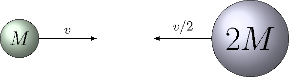
Fig. 11.7 Two colliding spheres

1. 0

2. \(3v/4\)

3. \(v\)

4. \(2v\)

5. \(3v\)

Answer: Since the two momentum vectors are equal in magnitude, but opposite in direction, the total momentum is the zero vector. Thus, this is their final momentum after the collision, giving a speed of zero.

11.4. 2D collisions

11.4.1. Example: Find final speeds

Let’s now try using conservation of linear momentum in two dimensions. The drawing below shows a collision between two pucks on an air-hockey table. Puck A has a mass of 23.0 g and is moving along the \(x\) axis with a speed of 5.50 m/s. It makes a collision with puck B, which has a mass of 63.0 g and is initially at rest. The collision is not head-on. After the collision, the two pucks fly apart with the angles shown in the drawing. The final speed of puck A is 3.38 m/s. Find the final speed of puck B (in m/s).

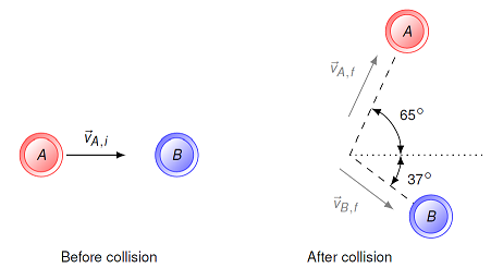
Fig. 11.8 Two colliding air-hockey pucks

To solve this problem, or any collision problem, our go-to method is momentum conservation. Thus, we start with the fact that the total momentum of the two-puck system stays the same before and after the collision.

\[ \sum {\vec p}_i = \sum {\vec p}_f \]

If we write out what this means in terms of the momenta for pucks A and B, we have

\[ {\vec p}_{A, i} + {\vec p}_{B, i} = {\vec p}_{A, f} + {\vec p}_{B, f} \]

Using \({\vec p} = m {\vec v}\) gives

\[ m_A {\vec v}_{A, i} + m_B {\vec v}_{B, i} = m_A {\vec v}_{A, f} + m_B {\vec v}_{B, f} \]

Puck B is not moving before the collision, so \({\vec v}_{B, i} = {\vec 0}\).

Now, to solve this vector equation, we need to break it up into its \(x\) and \(y\) components. Since there is no motion in the \(z\) direction, the \(z\) component of the total momentum is zero. This gives the two component equations

\[ x: m_A v_{A, ix} = m_A v_{A, fx} + m_B v_{B, fx} \qquad y: m_A v_{A, iy} = m_A v_{A, fy} + m_B v_{B, fy} \]

Puck A is chosen to move along the \(x\) axis before the collision, so \(v_{A, iy} = 0\). The figure shows the two directions for the final velocities; also, we know the final speed of puck A, and we are looking for the final speed of puck B. So it makes sense to use some trigonometry here, instead of writing the equations in terms of the velocity components. Using the vector diagrams

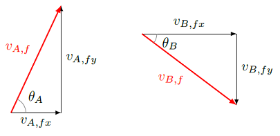
Fig. 11.9 Vector diagrams for \({\vec v}_{A, f}\) and \({\vec v}_{B, f}\)

we get that

\[ x: m_A v_{A, ix} = m_A v_{A, f} \cos \theta_A + m_B v_{B, f} \cos \theta_B\qquad y: 0 = m_A v_{A, f} \sin \theta_A - m_B v_{B, f} \sin \theta_B \]

Notice that the \(y\) component of the final velocity \({\vec v}_{B, f}\) is negative, so there is a corresponding minus sign in that equation.

We are solving for the final speed \(v_{B, f}\), which appears in both equations. Everything else in both equations is known, though, so we can really just pick one of the two, and solve for the unknown speed. Using the \(y\) equation, for example, gives

\[ v_{B, f} = \frac{m_A v_{A, f} \sin \theta_A}{m_B \sin \theta_B} = \biggl( \frac{m_A}{m_B} \biggr) \biggl( \frac{\sin \theta_A}{\sin \theta_B} \biggr) v_{A, f} \]

I have grouped together like quantities in the last equation. From this, we can easily see that if the masses have the same units, then it doesn’t matter what they are, since they cancel out. Similarly, the units we use for \(v_{A, f}\) will be the same as those for the final answer \(v_{B, f}\). Thus, we don’t have to convert from grams to kilograms when substituting here. In addition, we can see what happens if one mass is, say, four times the other, or the initial speed of puck A is halved. Algebraic equations can help answer questions like this easily without having to recalculate the entire problem. Plugging in the given values gives \(v_{B, f} = 1.858\) m/s.

Let’s now use these values to figure out the coefficient of restitution. Since this is a two-dimensional collision, there is more work to do here. Namely, we have to find the relative speed of the two pucks before and after the collision, by finding the magnitude of the difference in their velocities. Before the collision, this is easy, since

\[ {\vec v}_{A, i} - {\vec v}_{B, i} = (5.50 \textrm{ m/s}) {\hat x} \]

so that

\[ |{\vec v}_{A, i} - {\vec v}_{B, i}| = 5.50 \textrm{ m/s} \]

For after the collision, we need to find the two final velocities in unit vector form. We are given the final speed and direction of puck A, so its final velocity is

\[ {\vec v}_{A, f} = (1.428 \textrm{ m/s}) {\hat x} + (3.063 \textrm{ m/s}) {\hat y} \]

Using the final speed we just calculated for puck B, along with the given angle \(\theta_B\), we get (notice the minus sign in the \(y\) component!)

\[ {\vec v}_{B, f} = (1.485 \textrm{ m/s}) {\hat x} + (-1.119 \textrm{ m/s}) {\hat y} \]

Thus,

\[ {\vec v}_{A, f} - {\vec v}_{B, f} = (-5.70 \times 10^{-2} \textrm{ m/s}) {\hat x} + (4.182 \textrm{ m/s}) {\hat x} \]

Using the Pythagorean theorem with this vector difference, the relative speed of the two pucks after the collision is

\[ |{\vec v}_{A, f} - {\vec v}_{B, f}| = 4.182 \textrm{ m/s} \]

This gives the coefficient of restitution \(\epsilon\) is

\[ \epsilon = \frac{|{\vec v}_{A, f} - {\vec v}_{B, f}|}{|{\vec v}_{A, i} - {\vec v}_{B, i}|} = \frac{4.182 \textrm{ m/s}}{5.50 \textrm{ m/s}} = 0.760 \]

The collision is inelastic, but not completely inelastic.

11.4.2. Example: Smashing particles

Here, I show another example, where we are solving for one velocity, rather than one speed. The method I use will be different, and it is good to see this alternate technique. The drawing below shows a collision between two particles. The red particle has a mass of 200. g and is initially moving along the x-axis with a speed of 5.00 m/s. The blue particle has twice the mass of the red one and was initially at rest. After the collision, the red particle moves off with a velocity of 4.00 m/s at an angle of 54.9\(^\circ\) CCW from the +x-axis. What is the speed (in m/s) and direction (\(\theta_2\), or the angle CW from \(+x\) axis) of the blue particle after the collision?

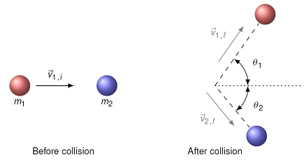
Fig. 11.10 Two colliding particles

The initial setup of this problem is much like the last example – we set up the conservation of momentum equations for the situation, making them particular for this situation. Thus,

\[ \sum {\vec p}_i = \sum {\vec p}_f \Rightarrow {\vec p}_{1, i} = {\vec p}_{1, f} + {\vec p}_{2, f} \]

The vector \({\vec p}_{2, i} = {\vec 0}\), since the second particle is initially at rest. Now we reach the point where we use a slightly different strategy than the last example. There, we knew the angle for puck B, so we could use trigonometry to write the momentum equations in terms of the unknown final speed \(v_{2, f}\). Here, though, we don’t know either the final speed or direction of the second particle. We could still use trigonometry as before, but if you try it, it can get a little messy. There is a smarter method, which is to write the unknown velocity in terms of its components, rather than its magnitude and direction. I can still write the final velocity for the first particle, using the known speed and direction. This gives the two equations

\[ x: m_1 v_{1, ix} = m_1 v_{1, f} \cos \theta_1 + m_2 v_{2, fx} \qquad y: 0 = m_1 v_{1, f} \sin \theta_2 + m_2 v_{2, fy} \]

The only change from the last example is how I wrote the last terms in each equation, keeping them as components, rather than using trigonometry. These can be solved for the unknown velocity components as

\[ v_{2, fx} = \biggl( \frac{m_1}{m_2} \biggr) (v_{1, ix} - v_{1, f} \cos \theta_1) \qquad v_{2, fy} = - \biggl( \frac{m_1}{m_2} \biggr) v_{1, f} \sin \theta_2 \]

As we would expect, \(v_{2, fy}\) is negative, since it moves downward. As the previous problem, I have written the masses separately from the rest. We have that \(m_1 / m_2 = 0.500\), since the blue mass \(m_2\) has twice the mass of the red one, so we didn’t even need to know the value of \(m_1\)!

Plugging in the given values, we calculate the components to be \(v_{2, fx} = 1.350\) m/s, and \(v_{2, fy} = -1.636\) m/s. Now, we can use the Pythagorean theorem to find the final speed, and the inverse tangent to find the direction. This gives a speed of 2.12 m/s, and an angle \(\theta_2\) (as given in the figure above) of \(50.5^\circ\).

Problem

Calculate the coefficient of restitution for the two particles in this collision. What type of collision is this?

Answer: \(\epsilon = 1.00\); the collision is elastic.

11.5. Summary

We have started using the ideas of center of mass and momentum in physical situations. For now, we have only covered what happens in a collision in a specific point of view, the center of mass frame of reference. Over the next few lessons, we will gradually look at more complicated situations.

After this lesson you should be able to:

• Calculate the center of mass position and velocity of a group of masses.

• Given a system in the CM frame of reference, calculate the unknown velocity before or after a collision, and the force on one of the objects due to the collision.

10. Linear momentum and Newton’s laws of motion 12. Solving force problems