.ipynb .pdf

Binder

Contents

18. Angular momentum

18.1. Overview

Links to programs in this lesson:

1. Angular momentum and linear motion

2. Angular momentum and central forces

3. Central forces and velocity components

In Lesson 11, the idea of linear momentum was introduced. Remember that this quantity is a good one to use when thinking about the inertia of an object. Linear momentum stays the same unless acted on by a net force (Newton’s 1st law); the size of the change in linear momentum is related to the size of this net force (Newton’s 2nd law). Thus, we could talk about the conservation of linear momentum when a system was isolated, i.e. no external forces acted on the system. Collisions were a good example of using this conservation principle to understand the motion of objects.

We will now go through an “angular” or “rotational” version of momentum. However, we will see that many of the same ideas hold here as they do with linear momentum – angular momentum changes due to the action of a net torque (or “rotational force”), while angular momentum is conserved in isolated systems. Perhaps surprisingly, this conservation of angular momentum works even if the object moves in a straight line! As long as we have a reference point (the \({\vec r} = 0\) location), we can calculate the angular momentum of an object around that point, regardless of what kind of motion the object has.

Angular momentum is very important in dealing with my favorite force: the gravitational force. Specifically, we can use conservation of angular momentum to talk about the orbit of one object around another (e.g. the Moon and the Earth). Indeed, it can be used for any central force, such as the spring force or the electrostatic force. Later on, we will also have discuss the principle of mechanical energy conservation, and between these two conservation principles, we can calculate quite a bit about an orbiting body. We will see a hint of that by the end of this lesson.

Here are the objectives for this lesson:

• Define torque and angular momentum.

• State the rotational version of Newton’s 2nd law.

• State the condition necessary for angular momentum to be conserved.

• Define point mass.

• Calculate the unknown mass, position, or perpendicular velocity component of a point mass using conservation of angular momentum.

18.2. Torque

Now that we have discussed the vector product in Lesson 17, we have enough of a mathematical framework to talk about torque. You should think of this as a rotational version of the force; we will use it primarily in these lessons to get some insight into angular momentum. Here is the definition of torque.

• Quantity: torque

• Symbol: \({\vec \tau}\) (“tau”)

• Equation:

\[ {\vec \tau} = {\vec r} \times {\vec F} \]

• Units: N \(\cdot\) m

Here \({\vec r}\) is the position where the force \({\vec F}\) acts; the position \({\vec r} = 0\) (sometimes called the “axis”) must be defined in order to find a torque. There are several consequences to this fact. For systems where the net force \(\sum {\vec F} \ne 0\), changing the position of the \({\vec r} = 0\) can give a different answer for the torque! So you should always specify the origin \({\vec r} = 0\) of the coordinate system when computing torques.

Forces are not torques

The torque \({\vec \tau}\) on an object can be zero, even if the force \({\vec F}\) creating the torque is not zero. This can occur if (1) the forces acts at the \({\vec r} = 0\) point, or (2) the force \({\vec F}\) is parallel to the position vector \({\vec r}\). Case (2) can be seen in the diagram below.

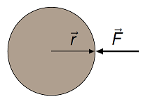
Fig. 18.1 Non-zero forces can give zero torques

Here, we have \({\vec \tau} = (R {\hat x}) \times (-F {\hat x}) = 0\).

The PhET linked below should help you build up some intuition about torques. Notice that, because the torque is related to both the force itself, and where the force acts, two forces of different sizes can cause the same magnitude of torque.

Let’s go through an example of finding the net torque vector for an object. Below is shown a cross-sectional view of a pulley with three forces acting on it at various points. The two pulley radii are 25.0 cm and 50.0 cm. The magnitudes of the forces are \(F_1 = 6.00\) N, \(F_2 = 12.0\) N and \(F_3 = 9.00\) N. We will find net torque on the pulley around its center, in unit vector notation.

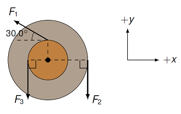
Fig. 18.2 Example of forces acting on a pulley to give a net torque

Since we are finding the net torque around the center, that will be our \({\vec r} = 0\) choice. I will call the smaller pulley radius \(r_1\), and the larger radius \(r_2\). Then, we can algebraically find the torques due to the various forces. The torques due to \({\vec F}_2\) and \({\vec F}_3\) are easier, so let’s do them first.

\[ {\vec \tau}_2 = (r_2 {\hat x}) \times (-F_2 {\hat y}) = (-r_2 F_2) {\hat z} \]

and

\[ {\vec \tau}_3 = (-r_1 {\hat x}) \times (-F_3 {\hat y}) = (r_1 F_3) {\hat z} \]

The torque \({\vec \tau}_1\) takes a little thought, since we have to be careful about our vectors. The force \({\vec F}_1\) is acting at a point \(r_1\) from the pulley’s center, along the \(+y\) axis. At this point, the force is 30.0\(^\circ\) CW from the \(-x\) axis. This means we have to break \({\vec F}_1\) into \(x\) and \(y\) components. With \(\theta = 30.0^\circ\), this gives

\[ {\vec \tau}_1 = (r_1 {\hat y}) \times [(-F_1 \cos \theta) {\hat x} + (F_1 \sin \theta) {\hat y}] = (r_1 F_1 \cos \theta) {\hat z} \]

You might be wondering why there is a \(\cos \theta\), since the magnitude formula we had before gave us \(|{\vec A} \times {\vec B}| = AB \sin \theta\). Here is a place where you have to watch out for the definitions! The angle \(\theta\) in \(AB \sin \theta\) is the angle between the vectors \({\vec A}\) and \({\vec B}\). However, for the pulley, the angle between the position vector \({\vec r}_1\) and the force vector \({\vec F}_1\) is not 30.0\(^\circ\), but rather its complement! This is why you get the cosine, rather than the sine, function. In other words, if you use the sine function, you would have to use \(\sin(90^\circ - \theta)\), which is the same as \(\cos \theta\).

Putting all of this together, we have

\[ \sum {\vec \tau} = {\vec \tau}_1 + {\vec \tau}_2 + {\vec \tau}_3 = (r_1 F_1 \cos \theta - r_2 F_2 + r_1 F_3) {\hat z} \]

Signs of the torques

In this case, where the position vector \({\vec r}\) and the force vector \({\vec F}\) are both in the \(x-y\) plane, notice how the signs are related to how each torque acts “around” the central point. Torques that tend to turn the object in the counterclockwise direction are positive, while those in the clockwise direction are negative. This is a shorthand way of finding the sign of the torque, without going through the full vector product calculation.

Substituting the numbers, we get \(\sum {\vec \tau} = (-2.45 \textrm{ N} \cdot \textrm{m}) {\hat z}\).

Problem

The length of the beam is 3.00 m, and the point \(C\) is at the center of the beam. What is the torque produced by the 10.0 N force around \(C\), in unit vector notation?

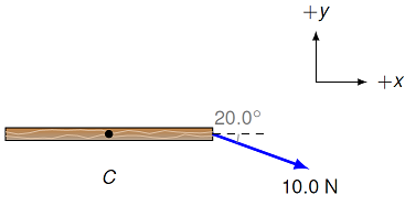
Fig. 18.3 Beam with a single force acting on it

Answer: \((-5.13 \textrm{ N m}) {\hat z}\)

Problem

The length of the beam is 3.00 m, with the point \(C\) at the center of the beam. Find the net torque (in N \(\cdot\) m) on the beam around an axis passing through point \(O\), and express your answer in unit vector notation.

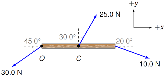
Fig. 18.4 Beam with multiple forces acting on it

Answer: \((22.2 \textrm{ N m}) {\hat z}\)

Problem

Below is shown a cross-sectional view of a pulley with three forces acting on it at various points. The two pulley radii are 1.00 cm and 2.50 cm. If the magnitudes of the forces are \(F_1 = 9.00\) N, \(F_2 = 10.0\) N and \(F_3 = 12.0\) N, what is the net torque (in mN \(\cdot\) m) on the pulley around its center, in unit vector notation?

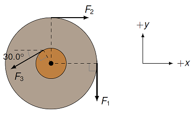
Fig. 18.5 Pulley with multiple forces

Answer: \((-355 \textrm{ mN m}) {\hat z}\)

18.3. Angular momentum

18.3.1. Angular momentum of point masses

Recall that in Lesson 11, linear momentum \({\vec p}\) was defined as

\[ {\vec p} = m {\vec v} \]

and from the same lesson, it changes whenever there is a net force acting on a system:

\[ \sum {\vec F} = \frac{\Delta {\vec p}}{\Delta t} \]

The intuition behind this is based on Newton’s 1st and 2nd laws of motion. The first law says that an object will move with a constant velocity unless acted on by an outside force. In terms of linear momentum, this says that the object (or system of objects) will have a constant \({\vec p}\) unless external forces are present. Newton’s second law then relates the net external force to the change in the system’s linear momentum.

In a similar manner, angular momentum \({\vec L}\) is a measure of the rotational motion of an object about a chosen axis. Much like Newton’s 2nd law says changes in linear momentum are due to net forces, there is a corresponding rotational version of this equation. Here, it says that changes in angular momentum are due to a net torque \({\vec \tau}\) acting on the system.

\[ \sum {\vec \tau} = \frac{\Delta {\vec L}}{\Delta t} \]

Again, this can be seen by our analogy between linear and rotational quantities. Here, we replace force with torque, \({\vec F} \to {\vec \tau}\), and linear momentum with angular momentum, or \({\vec p} \to {\vec L}\). This version of Newton’s 2nd law intuitively makes sense as torque changing the “spinningness” of an object, as represented by the angular momentum.

Symmetry gives conservation

The attentive reader may notice that I have tried to pull a fast one on you! Before, I said that conservation of linear momentum in the absence of net external forces is a re-statement of the principle of inertia (Newton’s 1st law). However, inertia only deals with constant velocity. As we saw when we discussed uniform circular motion, there is no corresponding “rotational” version of Newton’s 1st law – in other words, objects do not have a natural tendency to rotate, since this requires a centripetal force acting on the object. However, it turns out that the answer to this riddle deals with the symmetry of physics. One (slightly strange) way to say this is that if I took the entire Universe and rotated it, the laws of physics would be exactly the same – no one would notice! Modern physics is now based heavily on this idea of symmetry, based on the ideas of Emmy Noether, as discussed in the following videos linked here, and more in-depth here.

You would think from the name that angular momentum is only for rotating objects. But you would be wrong! It turns out that you can calculate the angular momentum of any object, whether they are rotating or not. In particular, for a point mass (i.e. an object whose size is much smaller than their distance away from the \({\vec r} = 0\) point), it is often helpful to use the following version of the angular momentum definition.

\[ {\vec L} = {\vec r} \times {\vec p} \]

where \({\vec p} = m{\vec v}\) is the linear momentum of the object. Consider a collection of masses \(m_i\), with an index \(i\). Then the total angular momentum \({\vec L}_{sys}\) of the system of masses \(m_i\) around a point \({\vec r} = 0\) would be given by

\[ {\vec L}_{sys} = \sum_i {\vec L}_i = \sum_i ({\vec r}_i \times {\vec p}_i) \]

Since each of the masses \(m_i\) has its own position \({\vec r}_i\) and linear momentum \({\vec p}_i\), the total angular momentum is the vector sum of the individual angular momenta. In addition, the change in this angular momentum with time is given by the net torque on the system, from Newton’s second law of rotational motion.

Problem

At a certain time, a 250. g object has a position vector \({\vec r} = (2.00 \textrm{ m}) {\hat x} + (-3.00 \textrm{ m}) {\hat y}\) and a velocity \({\vec v} = (5.00 \textrm{ m/s}) {\hat x} + (-4.00 \textrm{ m/s}) {\hat y}\). At that moment, a force \({\vec F} = (2.25 \textrm{ N}) {\hat y}\) is acting on the object.

1. What is the angular momentum of the particle at this instant?

2. What is the rate of change of the particle’s angular momentum?

Answers: \((1.75 \textrm{ kg m}^2 \textrm{/s}) {\hat z}\); \((4.50 \textrm{ kg m}^2 \textrm{/s}^2) {\hat z}\)

Problem

A particle with mass 2.00 kg is a distance \(r = 3.00\) m away from the origin, and moves with a speed \(v = 4.00\) m/s. A force \({\vec F}\) of magnitude 3.50 N acts on the particle. The vectors \({\vec r}, {\vec v}\) and \({\vec F}\) are all in the \(x-y\) plane as shown in the figure.

1. What is the angular momentum of the particle at the instant shown?

2. What is the rate of change of the particle’s angular momentum?

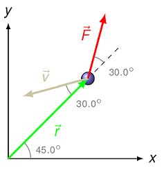
Fig. 18.6 Force acting on point mass

Answers: \((12.0 \textrm{ kg m}^2 \textrm{/s}) {\hat z}\); \((5.25 \textrm{ kg m}^2 \textrm{/s}^2) {\hat z}\)

18.3.2. Vector product tricks

Depending on the information you are given about a point mass, there may be easier ways to solve for the angular momentum of the mass. Let’s go through this in detail, especially since the same tricks can be used for anything that involves the vector product. The diagram below sets up the situation; the basic set-up and how to think about it are given below the picture.

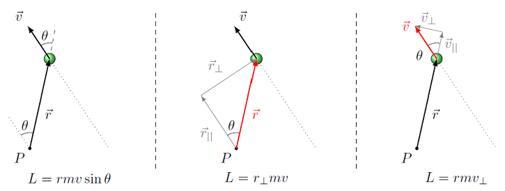
Fig. 18.7 Three perspectives on finding the magnitude of angular momentum

Suppose we are given a point mass moving at some velocity \({\vec v}\) along the dotted line, and it has a position \({\vec r}\) away from some special point \(P\). You are asked to find the magnitude of the angular momentum for the mass around \(P\). This is the situation in the left-hand diagram, where the velocity and position vectors are shown. At the mass, the line of the position vector is extended (this is the dashed line at the top), and the angle \(\theta\) between the two vectors \({\vec r}\) and \({\vec v}\) is shown. Then, we can use

\[ L = |{\vec r} \times {\vec p}| = |{\vec r} \times (m {\vec v})| = rmv \sin \theta \]

to find the magnitude, using this marked angle \(\theta\) along with the two magnitudes \(r\) and \(v\).

However, suppose we don’t know the entire vector \({\vec r}\). Sometimes you only know the distance between the point \(P\) and the line the mass moves along; I will call this distance \(r_\perp\). How would you solve the problem then? Looking at the middle picture, you can see that the position vector \({\vec r}\) has been broken up into its two components. One component \(r_{||}\) is in the same direction as the velocity \({\vec v}\), so it points parallel to the dotted line. The other component \(r_\perp\) is perpendicular to this line. If you look back at the left-hand diagram, you will see that there is a second dotted line, passing through the point \(P\), parallel to the motion of the mass. The two angles \(\theta\) are thus the same, since they are related by two parallel lines (the dotted lines) crossed by the same transversal (the position vector). This allows us to find the length of \(r_\perp\) as

\[ r_\perp = r \sin \theta \]

In the middle figure above, I have drawn the triangle so it uses the same angle \(\theta\) as the first picture. However, I can “slide” the distance \(r_\perp\) down to the point \(P\), and it will be the distance between \(P\) and the dotted line. This component \(r_\perp\) is a special one, so it has its own name – the moment arm: the shortest distance from the \({\vec r} = 0\) point to the line through the velocity vector of the object. Looking back at the magnitude of the angular momentum, we can use this moment arm to get

\[ L = rmv \sin \theta = (r \sin \theta) mv = r_\perp mv \]

So the angular momentum magnitude is the same as the moment arm \(r_\perp\) times the magnitude \(mv\) of the momentum (not a component of it!).

We can also play the same game if we only know the component \(v_\perp\) of the velocity perpendicular to \({\vec r}\). This is the right-hand picture in the diagram above. For example, if you imagine yourself watching a moving object, you actually only see \(v_\perp\) directly; the motion of the object towards or away from you is only apparent from the changing size of the object. Then, we can just use the angle \(\theta\) between \({\vec v}\) and \({\vec r}\) to divide the velocity into components parallel and perpendicular to the position vector – notice we are using “parallel” and “perpendicular” in a different sense than we did above with \(r_{||}\) and \(r_\perp\)! The component \(r_\perp\) is perpendicular to \({\vec v}\), while the component \(v_\perp\) is perpendicular to \({\vec r}\) . In any case, grouping the \(\sin \theta\) appropriately, this gives

\[ L = rmv \sin \theta = rm v_\perp \]

We will see this version of the angular momentum mangitude often when we treat orbits, such as the orbit of a planet around a star. Cases like this will be discussed in Lesson 23 (Kepler’s laws).

Problem

For the diagram below, you have already found the angular momentum of the particle in an earlier problem.

Fig. 18.8 Force acting on point mass

1. What is the magnitude (in m/s) of the velocity component \(v_\perp\) perpendicular to the position vector \({\vec r}\)?

2. What is the magnitude (in m) of the position component \(r_\perp\) perpendicular to the velocity vector \({\vec r}\)? In other words, what is the moment arm of the mass?

Answers: 2.00 m/s; 1.50 m

Obviously, point masses are not the only types of object that occur in physics. As mentioned above, for extended objects, we can use conservation of angular momentum to find, for example, the rotational speed of an object. However, this depends on defining a quantity known as the moment of inertia. Much like mass is a measure of an object’s resistance to linear motion, the moment of inertia is the same for rotational motion. However, we will not define this quantity because we are focusing on the angular momentum of point masses. You may see the moment of inertia in a future physics class, when you are dealing with the rotation of an extended object.

18.3.3. Angular momentum in vPython

We will now delve further into the notion of angular momentum using vPython. The program below creates a ball moving with a constant velocity. Thus, the ball will move along the line \(r_y = +2\) at constant speed \(v = 1\). The ball is also given a mass M, defined at the beginning of the program. In addition, there are two arrows in the simulation: a yellow arrow showing the constant velocity \({\vec v}\) of the ball, and a cyan arrow showing the changing ball position \({\vec r}\). Run the program, and note how \({\vec r}\) and \({\vec v}\) change with time.

Back to program list

Now you will need to calculate the magnitude \(L\) of the angular momentum, and graph this magnitude as a function of time. \(L\) is calculated from the position \({\vec r}_O = (0, 0, 0)\). In other words, the vector difference \(\Delta {\vec r} = {\vec r}_b - {\vec r}_O\) between the ball’s position \({\vec r}_b\) and the origin \({\vec r}_O\) will be used to define the angular momentum \({\vec L}_b = \Delta {\vec r} \times {\vec p}\) of the mass.

Problem

As the ball moves in the \(x-y\) plane, its angular momentum vector will have a non-zero component only in one direction. What is that direction?

Answer: Since \(\Delta {\vec r}\) will have only \(x\) and \(y\) components, and \({\vec v}\) only has a \(y\) component, then \({\vec L}\) will only have a \(z\) component. All other components of \({\vec L}\) are zero, since neither \(\Delta {\vec r}\) nor \({\vec v}\) have \(z\) components.

The steps to do this are similar to those you have used with previous lessons; Lesson 03 would be a useful reference. In the space indicated just before the evolution loop, create a graph angMomGraph. Set its horizontal axis limits as xmin = 0 and xmax = MAX_TIME. Also, set its lower vertical axis limit as ymin = 0. Label the two axes with proper titles using xtitle and ytitle (including units!). Immediately below this, create a blue curve angMomCurve using the graph angMomGraph. In the space indicated inside the evolution loop, update the angular momentum graph by plotting the appropriate component of the angular momentum at the time \(t\). Use the definition of angular momentum, along with the modules cross, to find the component of \({\vec L}\) you are plotting.

Once you have done all of the coding above, run the program and see what the \(L\) vs. \(t\) graph looks like; you should get something like the graph shown below. What is true about the magnitude of the angular momentum for the ball? This demonstrates that angular momentum can be used for objects that have no “rotational” aspect to their motion.

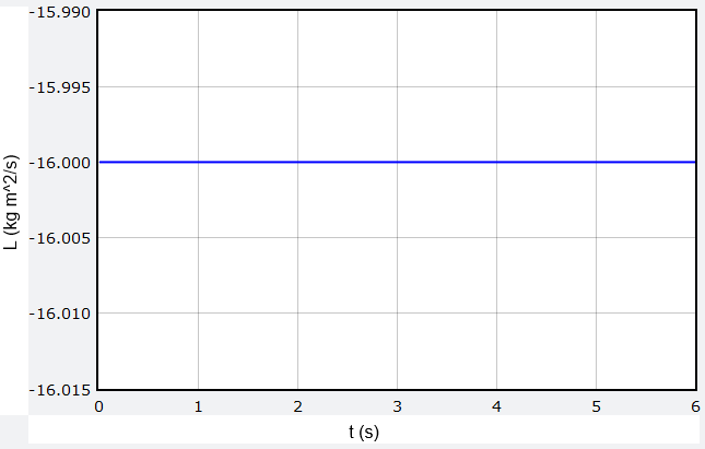
Fig. 18.9 Graph of \(L_z\) vs. time for the moving ball

Problem

What would be the angular momentum of the ball if it started at \({\vec r}_{b, i} = (-3, -2, 0)\) – in other words, it travels along a line \(r_y = -2\) instead of \(r_y = +2\)? Keep the velocity the same as before. Calculate this yourself first, then change the code above to verify your answer. Has anything changed with the magnitude and direction of \({\vec L}\)?

Answer: The angular momentum vector \({\vec L} = (+16.0 \textrm{ kg m/s}) {\hat z}\). The magnitude of the angular momentum is the same, but the direction of \({\vec L}\) has reversed.

Problem

What would be the angular momentum of the ball if it traveled along the line \(r_y = 0\)? Keep the velocity the same as before. Calculate this yourself first, then change the code above to verify your answer.

Answer: The angular momentum vector \({\vec L}\) is now the zero vector.

Use the intuition you have gained from the vPython simulation to answer the following question.

Problem

The figure shows three particles, all moving in the same direction along straight lines. Particle 3 moves directly away from point \(P\), while the trajectories of the other two have the moment arms as shown. All three particles have the same mass and speed. Rank the magnitudes of the angular momenta of the three particles around the point \(P\).

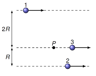
Fig. 18.10 Rank the angular momenta magnitudes of the point masses

Answer: \(1 > 2 > 3\)

18.3.4. Conservation of angular momentum

Recall that in Lesson 11, we saw that when the net force on a system was zero, this meant the momentum of that system remained constant (or was conserved):

\[ \sum {\vec F} = \frac{\Delta {\vec p}}{\Delta t} = 0 \Rightarrow \Delta {\vec p} = 0 \]

Similarly, if the net torque acting on a system is zero, then the angular momentum of the system is conserved as well.

\[ \sum {\vec \tau} = \frac{\Delta {\vec L}}{\Delta t} = 0 \Rightarrow \Delta {\vec L} = 0 \]

Remember that a zero net torque does not mean a zero net force!

Problem

A 2.00 kg red bowling ball, moving to the right at a speed of 3.00 m/s on a frictionless table, collides head-on with a stationary 3.00 kg green bowling ball. The green ball leaves the collision at 2.67 m/s to the right. The two balls move along a line that is a distance \(L\) of 1.50 m from a marked point \(P\). Give your answers in unit vector notation.

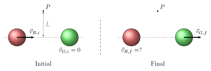
Fig. 18.11 A red ball strikes a sationary green ball

1. What is the initial angular momentum (in kg m\(^2\)/s\(^2\)) of the green ball around the point \(P\)?

2. What is the initial angular momentum (in kg m\(^2\)/s\(^2\)) of the red ball around the point \(P\)?

3. What is the final angular momentum (in kg m\(^2\)/s\(^2\)) of the green ball around the point \(P\)?

4. Using conservation of angular momentum, find the final velocity (in m/s) of the red ball. Think carefully about how to go from the final angular momentum of the red ball, to its final velocity.

Answers: \((6.00 \textrm{ kg m}^2 \textrm{/s}^2) {\hat z}\); \((0.00 \textrm{ kg m}^2 \textrm{/s}^2) {\hat z}\); \((12.0 \textrm{ kg m}^2 \textrm{/s}^2) {\hat z}\); \((-2.00 \textrm{ m/s}) {\hat x}\)

A classic physics demonstration dealing with the conservation of angular momentum is to hang a bicycle wheel off of a rope on one side. If the wheel is not spinning, then once you let go of the wheel, it will drop to point downward as you would expect. However, it does something very surprising if the wheel is spinning! This is detailed in the video linked below, from the Veritasium YouTube channel, always a good source of science videos. In the video, the channel Smarter Every Day is also mentioned, since this video relates to a series on helicopter physics on that other channel – well worth checking out!

Challenge

There is one small error in this video. Did you see it?

18.4. Central forces

18.4.1. An alternative definition

We talked about central forces in Lesson 16.6; examples of these are the prominent forces of gravitation, the spring force, and the electrostatic force. In that previous lesson, we defined a central force \({\vec F}_c\) as a force of the form

\[ {\vec F}_c = F_c (-{\hat r}) \]

Here, \({\vec r}\) is the position of the object acted on by the force, so \({\hat r}\) is the associated unit vector. Now that we have talked about the vector product and torque, we can phrase this condition in another, equivalent manner. A central force is a force that exerts no torque about the central point \({\vec r} = {\vec 0}\). Below is a repeat of the picture you saw in Lesson 18, where I first introduced central forces.

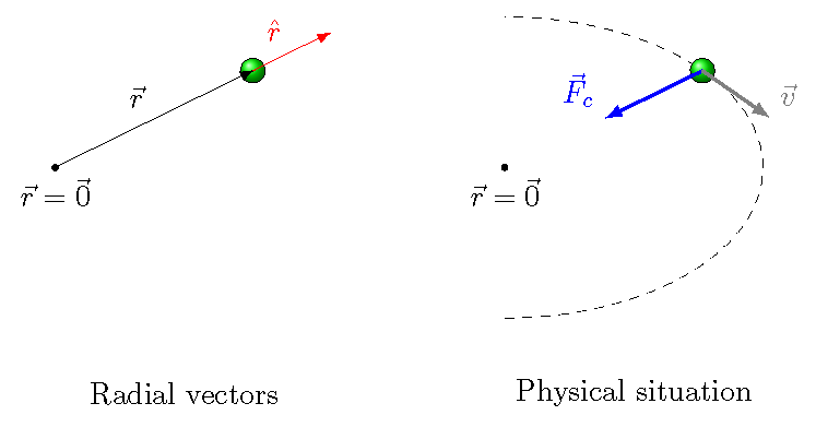
Fig. 18.12 The radial vectors and the physical situation for a central force

Central forces and net torque

A central force \({\vec F}_c\) is a force which gives no net torque around the point \({\vec r} = {\vec 0}\). In other words,

\[ {\vec \tau} = {\vec r} \times {\vec F_c} = {\vec 0} \]

Why are these the same? It boils down to the fact that the unit vector \({\vec r}\) is along the same line as the unit vector \({\hat r}\), so their vector product is zero:

\[ {\vec r} \times {\vec F_c} = (-F_c) ({\vec r} \times {\hat r}) = {\vec 0} \]

Let’s work through this in detail, to see how it goes. The position vector in unit vector form is

\[ {\vec r} = r_x {\hat x} + r_y {\hat y} + r_x {\hat z} \]

Using the three-dimensional Pythagorean theorem to find the magnitude \(r\) of this vector, then \({\hat r} = {\vec r} / r\), or

\[ {\hat r} = \biggl( \frac{r_x}{r} \biggr) {\hat x} + \biggl( \frac{r_y}{r} \biggr) {\hat y} + \biggl( \frac{r_z}{r} \biggr) {\hat z} \]

Then the central force is written as

\[ {\vec F}_c = \biggl( -\frac{r_x F_c}{r} \biggr) {\hat x} + \biggl( -\frac{r_y F_c}{r} \biggr) {\hat y} + \biggl( -\frac{r_z F_c}{r} \biggr) {\hat z} \]

Putting this all together, the vector product of the position vector and the force gives

\[ {\vec r} \times {\vec F_c} = \biggl[ \frac{(r_y r_z - r_z r_y) F_c}{r} \biggr] {\hat x} + \biggl[ \frac{(r_z r_x - r_x r_z) F_c}{r} \biggr] {\hat y} +\biggl[ \frac{(r_x r_y - r_y r_x) F_c}{r} \biggr] {\hat z} \]

Thus, every term cancels out, and the entire vector product is just the zero vector.

Problem

Which of the following forces are a central force? In each choice, the letters \(A, B, C, D\) represent constants; \({\vec r}\) is the position vector of the object acted on by the force, and \({\hat r}\) is the unit vector pointing in the same direction as the position vector.

1. \({\vec F}_1 = -A {\vec r}\)

2. \({\vec F}_2 = (B r_x) {\hat y}\)

3. \({\vec F}_3 = (C / r^2) {\hat r}\)

4. \({\vec F}_4 = D[(-r_y) {\hat x} + (r_x) {\hat y}]\)

Answer: Only \({\vec F}_1\) and \({\vec F}_3\) are central forces.

Problem

Write a vPython function isCentralForce() which determines whether a force acting at a particular position could be a central force. Assume that a force \({\vec F}\) is acting on an object currently at position \({\vec r}\). Then, the arguments of isCentralForce() are two vPython vectors – forceVec representing the force \({\vec F}\), and posVec representing the position \({\vec r}\). The function should return True if the force could be a central force, and False otherwise.

Answer: Here is a possible solution.

def isCentralForce(forceVec, posVec):
    '''
    Use definition of central force as one where
    net force on object due to force is zero.
    '''
    
    if cross(posVec, forceVec) == vector(0, 0, 0):     # Net torque is zero vector
        return True
    else:                                              # Non-zero net torque
        return False

Since the constant central force here produces no torque on the orbiting object, this means the angular momentum of the object is conserved. This comes from Newton’s second law of rotational law, namely

\[ \sum {\vec \tau} = \frac{\Delta {\vec L}}{\Delta t} = 0 \Rightarrow \Delta {\vec L} = 0 \]

This is true of all central forces, since they all have zero net torque.

Central forces and angular momentum

A force will conserve angular momentum only if it is a central force.

18.4.2. Central force simulation

Let’s now create a vPython simulation of a point mass acted on by this constant central force. Below is the same code we saw in Lesson 16 the last time we talked about central forces; the only addition is that a graph of the angular momentum component in the \(z\) direction has been added.

Problem

Before you run the program, using the physical parameters defined in the code, calculate the angular momentum vector of the ball. Remember you can look at the code by clicking on the pencil icon in the Trinket app.

Answer: \((60.0 \textrm{ kg m}^2 \textrm{/s}^2) {\hat z}\)

Back to program list

When you run the program above, you will see that the \(z\) component \(L_z\) of the angular momentum will “wobble” around a little bit (due to numerical error), but that the value basically stays the same. I am using a pretty simple updating scheme, so this is pretty good; other, more sophisticated, methods would give even better results.

However, this is not the normal situation! Remember that we have specified a constant central force. Whenever the force is not a central force – i.e. whenever it produces a net torque on the object – then the angular momentum will not stay constant. To see an example of this, you will use the program above, but change the force. In particular, use the force given by

\[ {\vec F} = F_c (-r_y {\hat x} + r_x {\hat y}) \]

You will need to change the two commands in the program where ball.force is defined to the appropriate code; you can keep the constant FORCE_MAG in front. After you have made the changes, run the program. You should notice a dramatic change in the value of \({\vec L}\)! The object will spiral outward from the center with increasing speed and radius. This is because the force acting on the object is always acting tangent to the position vector, and so increases the object’s “spinningness” always in the same direction. Thus, a net torque is always created in one rotational direction (which depends on how you put in the signs).

18.4.3. Example: Calculating the parallel velocity component

Let’s now use conservation of angular momentum to find how the velocity changes as the ball moves in the original simulation. So, if you changed the force, change it back to \({\vec F}_c = -F_c {\hat r}\). For the default values given in the program above, the initial position of the ball is at its largest radius from the center. Let’s see why that is true; this will recount some of our discussion from Lesson 16. To start, the ball is moving perpendicular to its position vector, so the velocity has a zero radial component. Then, we can compare the net force on the ball to the necessary centripetal force needed to keep it at that radius. Plugging in the default numbers from the program above, we get

\[ F_{cp} = \frac{mv^2}{r} = 1.44 \textrm{ N} \]

This is much smaller than the constant 10.0 N of the central force \({\vec F}_c\), so the ball will move inward under the central force. If \(F_{cp}\) had been the same as \(F_c\), the ball would have moved in the same radius all the time. If \(F_{cp}\) was larger than \(F_c\), the ball would have been moving too fast to stay at that radius, and moved outward. Although we haven’t talked about it yet in class, you can then use conservation of mechanical energy (Lesson 20) that the ball will never go to a larger radius than its initial one.

It may help to see how the radius of the object changes with time, and compare that to the sizes of the radial and perpendicular velocity components. This is done in the program below. To flesh this out, I should emphasize that I only used the scalar product to find these components, not the angular momentum! However, obviously these should match up in the end, and they do, as we will see. To find the radial velocity component \(v_r\), I used the fact that this is the component in the same direction as the position unit vector \({\hat r}\), so that

\[ v_r = {\vec v} \cdot {\hat r} \]

I used \({\hat r}\), rather than \({\vec r}\), so that I do not have to divide out by the magnitude \(r\) of the position vector to get just \(v_r\). Then, the perpendicular velocity component \(v_\perp\) is what is left over, given by the magnitude

\[ v_\perp = |{\vec v} - v_r {\hat r}| \]

This explains why I used the particular vPython commands in the program below. Run the program, and watch how \(v_r\) (the red curve) and \(v_\perp\) (green curve) vary with the radius \(r\) (the blue curve).

Back to program list

After the program has run, you can use the cursor over the graph to find the smallest radius is 4.03 m; this is the value when the blue line is at one of its “dips”. We will now use angular momentum to find the speed of the ball at this radius. The key point is to realize that, just like at the maximum radius, when the ball is at its minimum radius, it has stopped moving towards the center. Thus, the radial component of the velocity \(v_r = 0\); you can see these are the points where the red line passes through a value of zero. Said a different way, the speed of the ball at this smallest radius is equal to the perpendicular velocity component \(v_\perp\). But this is exactly what appears in the angular momentum! In fact, we can say that, with angular momentum conservation,

\[ L_i = L_f \Rightarrow r_i m v_{i, \perp} = r_f m v_{f, \perp} \]

With \(r_i\) the largest radius and \(r_f\) the smallest, we can solve for the speed \(v_{f, \perp}\) at the smallest radius with some algebra, to get

\[ v_{f, \perp} = \biggl( \frac{r_i}{r_f} \biggr) v_{i, \perp} \]

Notice what is happening here. Since \(r_i > r_f\), then \(v_{f, \perp} > v_{i, \perp}\); at the larger radius \(r_i\), the ball has a smaller speed \(v_{i, \perp}\), while at the smaller radius \(r_f\), the speed \(v_{f, \perp}\) is larger. Conservation of angular momentum says that the perpendicular velocity component \(v_\perp\) is larger as the radius gets smaller. We can verify this by plugging in the numbers to get \(v_{f, \perp} = 3.72\) m/s, larger than the initial speed of 3.00 m/s. You can use your cursor on the green curve of the graph to confirm this is the correct value.

Angular momentum depends only on \(v_\perp\)

One crucial part of the analysis above is taking the radius of the ball when it is at the closest to, or furthest away, from the center. These are the only locations when \(v_r = 0\). At all other radii, this is not true, and the angular momentum only gives the perpendicular component \(v_\perp\) of the total velocity. This is shown in the figure below, where the ball is at three different locations – the maximum radius \(r_{max}\), the minimum radius \(r_{min}\), and an intermediate value \(r\) of the radius. Only for the middle value of \(r\) do you have a non-zero radial velocity component \(v_r\). At this middle location, you cannot use angular momentum conservation to find the speed of the object, just its component \(v_\perp\).

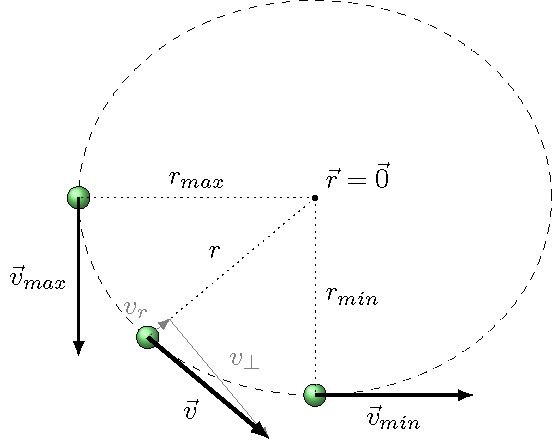
Fig. 18.13 Three possible radii for the object moving in a central force, and their associated velocity vectors

Remember that the speed \(v\) of the ball is given in terms of the components \(v_r\) and \(v_\perp\) by the Pythagorean theorem:

\[ v^2 = v^2 _r + v^2 _\perp \]

So if you know one of \(v\) or \(v_r\), as well as the angular momentum (to get \(v_\perp\)), you can find the other value.

Problem

When the ball is at a radius halfway between the largest and smallest values (i.e. \(r = 4.52\) m), the computer tells you its speed is 3.38 m/s. What is the size of the radial velocity component \(v_r\) (in cm/s) of the ball at this radius?

Answer: 62.3 cm/s

18.5. Summary

In this lesson, we see another rotational quantity that has its analogue in linear motion. Just as torque is similar (but not the same as!) force, the angular momentum of an object is similar to its linear momentum. Each pair of physical quantities are related, but the addition of the position vector \({\vec r}\) and the vector product are an extra element that you need to consider. The analogy goes on to relate net torque and angular momentum with the rotational version of Newton’s second law (just as we saw in Lesson 11 between net force and linear momentum).

We also saw that the angular momentum of a system remains the same when the net torque on that system is zero. Such conservation laws are an important tool in physics, and the conservation of angular momentum is no exception. In fact, when combined with the conservation of mechanical energy, these two principles will go far in describing the motion of an orbiting body when considering Newton’s law of universal gravitation.

After this lesson, you should be able to:

• Define angular momentum, either for a generic object or for a point mass.

• Calculate the angular momentum of an object around a given point \({\vec r} = {\vec 0}\).

• Explain when angular momentum is conserved.

• Use conservation of angular momentum to calculate the mass or speed of an object.

17. Vector product 19. Work and energy