.ipynb .pdf

Binder

Contents

21. Universal gravitation

21.1. Overview

Link to the program in this lesson:

1. Net gravitational force on an object

The gravitational force played an important role in the history of physics. It was in Newton’s seminal book, known today as the Principia, where he worked out the implications of his laws of motion, and one of the pivotal cases was that of the Moon’s orbit around the Earth. This provided the first evidence that motion near the Earth’s surface, and motion of objects in the sky, obeyed the same physical laws. This was a game changer in the world of ideas, and led to the mathematical framework for an understanding of the Universe we now call “physics”.

Before, Newton, in the Western scientific tradition one of the earliest influential theories of why objects fall towards the Earth was developed by Aristotle (in the 4th century BC), who thought that all substances have a natural place in the Universe (with the Earth at its center), and objects will move to this place based on their composition. There is no gravitational force yet! The Indian astronomer and mathematician Brahmagupta in the 7th century wrote about an actual force of attraction between the Earth and other objects, pulling them towards the Earth’s surface. He saw the Earth as a sphere, and that the attraction would be the same for all points on the surface.

As we will talk more about in Lesson 23, in the early 17th century Johannes Kepler used new astronomical observations to deduce the motions of the planets based on the idea of having the Sun at the center of the Solar System. In that lesson, we will show how Newton’s law of universal gravitation – developed in this lesson – leads to a description of planetary motion in the Solar System.

Sir Isaac Newton formulated a notion of a gravitational force between two objects which acts along the line between them, based on an idea of Robert Hooke and others. Using this gravitational force, Newton was able to explain why Kepler’s laws of planetary motion worked. A key part of the process was Newton’s realization that the force of gravity pulling objects towards the Earth is exactly the same force as that keeping the Moon in orbit around the Earth, and both in orbit around the Sun.

Here are the objectives for this lesson:

• State Newton’s law of universal gravitation.

• State the definition of gravitational field.

• Find the gravitational force acting on a single mass due to a group of surrounding masses.

• Find the gravitatational field at a given distance away from a known mass.

21.2. The gravitational force equation

21.2.1. Notation review

In order to write down Newton’s law of universal gravitation, it may be helpful to review some notation; this is similar to notation we defined back in Lesson 02 when we first looked at relative position vectors. First, remember that an object’s position is defined by a vector \({\vec r}\), which points from the origin (i.e. \({\vec r} = {\vec 0}\)) to the object. For more than one object, we can label these position vectors as we do the objects, as seen in the diagram below. In this diagram, there are two objects, \(m_1\) and \(m_2\), with corresponding position vectors \({\vec r}_1\) and \({\vec r}_2\).

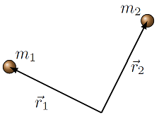
Fig. 21.1 Position vectors for two objects

Now, suppose we want to define an interaction between the two objects, which does depend on our choice of origin, but only the relative position of the objects. This is what is needed for central forces, such as the gravitational force (for this lesson) as well as the electrostatic force (in Lesson 24 for Coulomb’s law). In both of these cases, the direction of the force is on the line connecting the two objects, either towards the other object (for attractive forces) or away (for repulsion). The choice of origin should not matter – these forces are the same, regardless of how the coordinates are picked. To this end, we can define the relative position vectors

\[ {\vec r}_{12} = {\vec r}_1 - {\vec r}_2 \qquad {\vec r}_{21} = {\vec r}_2 - {\vec r}_1 \]

This means that the vector \({\vec r}_{ij}\) is the vector with its tip at object \(i\), and its tail at object \(j\). You may want to look back at Lesson 02 to remind yourself of graphical vector addition, in order to see where the directions of the vectors come from. Because of these definitions, \({\vec r}_{12} = -{\vec r}_{21}\).

However, all we care about now is the direction, not the magnitude of the distance between these objects. So we take these vectors \({\vec r}_{ij}\), and find the unit vector pointing in the same direction. Remember from Lesson 07 that this would be defined as

\[ {\hat r}_{ij} = \frac{{\vec r}_{ij}}{r_{ij}} \]

where, as usual, \(r_{ij}\) is the magnitude of the vector \({\vec r}_{ij}\). Notice that this means the units cancel out! The unit vector \({\hat r}_{ij}\) summarizes where the object \(i\) is, as seen by object \(j\). It is helpful to think of each unit vector \({\hat r}_{ij}\) with its tail at object \(i\), and pointing away from object \(j\). This is shown in the diagram below, along with the position vectors from the last figure.

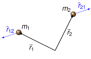
Fig. 21.2 The unit vectors \({\hat r}_{ij}\)

Problem

Suppose that object 1 is at position \((1.25 \textrm{ m}) {\hat x} + (-75.0 \textrm{ cm}) {\hat y}\) and object 2 is located at \((65.0 \textrm{ cm}) {\hat x} + (35.0 \textrm{ cm}) {\hat y}\).

1. What is the unit vector \({\hat r}_{12}\) at object 1 pointing away from object 2?

2. What is the unit vector \({\hat r}_{21}\)?

Answers: \({\hat r}_{12} = 0.479 {\hat x} - 0.878 {\hat y}\); \({\hat r}_{21} = -0.479 {\hat x} + 0.878 {\hat y}\)

Problem

Write a vPython function rHat() that calculates the unit vector \({\hat r}_{ij}\) at an object \(i\) with position \({\vec r}_i\), away from an object \(j\) at position \({\vec r}_j\). The two arguments of the function are r_i and r_j, which are vPython vectors representing the vectors \({\vec r}_i\) and \({\vec r}_j\), respectively. The function should return the unit vector \({\hat r}_{ij}\). See if you can do this without using the built-in vPython modules mag() or hat()! You will need to use the square root function sqrt(), however.

Answer: Here is one possible program.

def rHat(r_i, r_j):

    # Find relative position vector
    
    rel_pos = r_i - r_j
    
    # Find magnitude of this vector
    
    r_mag = sqrt(rel_pos.x ** 2 + rel_pos.y ** 2 + rel_pos.z ** 2)
    
    # Return unit vector r_ij
    
    return rel_pos / r_mag

21.2.2. The universal force of gravitation

Using the definition of the unit vector \({\hat r}_{ij}\), we can now write down Newton’s law of universal gravitation. This gives the gravitational force between two point masses \(m_i\) and \(m_j\) as

\[ {\vec F}_{g, ij} = -\biggl( \frac{G m_i m_j}{r^2 _{ij}} \biggr) {\hat r}_{ij} \]

with the constant \(G = 6.67 \times 10^{-11}\) N\(\cdot\)m\(^2\)/kg\(^2\).

There are several things to unpack in this equation. This quantity \({\vec F}_{g, ij}\) is the gravitational force on object \(i\), due to object \(j\); this ordering matches our definition of the unit vector \({\hat r}_{ij}\) at the mass \(i\). If we flip the ordering of \(i\) and \(j\), we flip the sign of the unit vector, while everything else stays the same, so that \({\vec F}_{g, ji} = -{\vec F}_{g, ij}\). Both masses \(m_i\) and \(m_j\) appear in exactly the same way in the equation, i.e. you can reverse them and get the same magnitude, although as stated in the last point, the direction would reverse. This is what we would expect from Newton’s third law.

The size of the force depends on the inverse of the square of the center-to-center distance \(r_{ij}\) between the two masses. This is known as an inverse square law. The force magnitude gets smaller as the distance gets larger, and vice versa. The electrostatic force is another example of an inverse square law. For physics in three spatial dimensions, an inverse square law is a sure sign of a force that has an infinite range!

Finally, the sign in front of the equation is probably confusing. If we look at the grouping \(-{\hat r}_{ij}\), we see that the gravitational force on mass \(i\) always points towards mass \(j\); the force is attractive. Said differently, since \({\hat r}_{ij}\) always points away from the other mass, the minus sign tells us the force points towards the other mass. Note that this depends on the rest of the equation being positive! We will see a very similar form for the electrostatic force in Lesson 24(Coulomb’s law), but since electric charges can be negative, the electrostatic force can be either attractive or repulsive.

Problem

Consider the two masses shown in the figure below. When the two masses 1 and 2 have the same size \(M\), the magnitude of the gravitational force on mass 1 is 3.00 N. If we replace one mass with a mass 1\(^\prime\) of size \(4M\) (as shown in the lower part of the figure below), what is the magnitude of the force \(F_{1^\prime}\) on the new mass 1\(^\prime\), due to the old? Choose the best answer below.

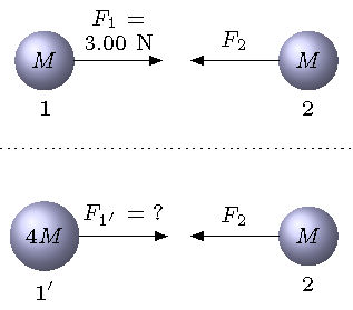
Fig. 21.3 Original situation on top, and the new situation on bottom

1. 0.750 N

2. 3.00 N

3. 12.0 N

4. 16.0 N

5. 48.0 N

Answer: 12.0 N

Problem

The force between two masses separated by a distance \(d\) is \(F\). If the masses are pulled apart to a distance \(3d\), what is the new magnitude of the gravitational force on each mass? Choose the best answer below.

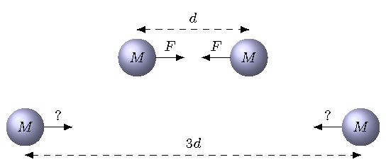
Fig. 21.4 Two attracting masses

1. \(9F\)

2. \(3F\)

3. \(F\)

4. \(F/3\)

5. \(F/9\)

Answer: \(F/9\)

21.2.3. An example: masses in an equilateral triangle

Let’s work through an example, to see how to calculate the gravitational force; we will also see how the unit vectors \({\hat r}_{ij}\) are used. In the figure below, three masses are held in place at the corners of an equilateral triangle with sides \(d\) of 7.00 m. The sizes of the three masses are \(m_1 = 2.00\) kg, \(m_2 = 4.00\) kg, and \(m_3 = 3.00\) kg. We are going to find the net gravitational force acting on the top mass \(m_1\), due to the other two masses.

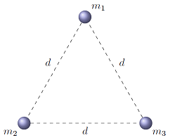
Fig. 21.5 Three masses fixed at the corners of an equilateral triangle

As usual for force problems, our first step is to draw the FBD for the object whose net force we are calculating. This is shown below.

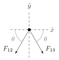
Fig. 21.6 FBD for mass \(m_1\)

where \(\theta = 60.0^\circ\). Again, make sure you are good with the notation here – \({\vec F}_{12}\) is the gravitational force on mass 1 due to mass 2, while \({\vec F}_{13}\) is the gravitational force on mass 1 due to mass 3. On the other hand, \({\vec F}_{21}\) is the force on mass 2 due to mass 1, which is related to \({\vec F}_{12}\) by Newton’s third law, but not the same. We can also label the two angles for each force with the same symbol \(\theta\), since the masses are on the corners of an equilateral triangle. This is not true in general!

Make sure you find the right forces

You may remember that when we first talked about Newton’s laws of motion in Lesson 11, I introduced them with a “zeroth law”. This law says that an object responds only to the forces acting directly on it. At the time, most of you probably said this is common sense, and why do I need to spell this out? Well, here’s the reason! My experience when starting with gravitational force (or electrostatic forces in Lesson 24) is that students get confused about the directions of the forces, because they are not taking Newton’s zeroth law into account! We only care about the forces acting on mass 1. I often see students answering questions like this by telling me about the forces on \(m_2\) and \(m_3\); those are irrelevant! Find out how the masses act on mass 1, not how mass 1 acts on the other masses.

To calculate the force vectors \({\vec F}_{12}, {\vec F}_{13}\), we need the unit vectors \({\hat r}_{12}, {\hat r}_{13}\). In the end, the arrows we have already drawn in the FBD should match those we are about to get from using the gravitational force equation – this is something you should check! Fortunately, since we know the relative positions of each mass, we do not have to do too much calculation here. The important thing to remember is that these two unit vectors always point from the other two masses. You can see the unit vectors superimposed on the physical situation in the figure below.

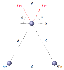
Fig. 21.7 Unit vectors \({\hat r}_{12}\) and \({\hat r}_{13}\)

Therefore, the unit vectors are given by

\[ {\hat r}_{12} = (\cos \theta) {\hat x} + (\sin \theta) {\hat y} \qquad {\hat r}_{13} = (-\cos \theta) {\hat x} + (\sin \theta) {\hat y} \]

These vectors came from seeing which quadrant they were in, knowing the angle \(\theta\), plus the fact that unit vectors have a magnitude of 1. For this problem, that was the hard part! The rest is just substituting into the gravitational force equation. Let’s find the force \({\vec F}_{12}\) first. This would be

\[ {\vec F}_{12} = -\biggl( \frac{G m_1 m_2}{r^2 _{12}} \biggr) {\hat r}_{12} = \biggl(\frac{G m_1 m_2}{d^2} \biggr) [(-\cos \theta) {\hat x} + (-\sin \theta)] \]

In the second equality, I have taken the minus sign from out front, and distributed it over the components of \({\hat r}_{12}\). Thus, the direction of this vector is in the third quadrant, since both the \(x\) and \(y\) components are negative. This matches what we drew for \({\vec F}_{12}\) in the FBD! I also used the fact that the distance \(r_{12}\) is simply the side length \(d\) of the triangle. Similarly, for \({\vec F}_{13}\), we have

\[ {\vec F}_{13} = -\biggl( \frac{G m_1 m_3}{r^2 _{13}} \biggr) {\hat r}_{13} = \biggl(\frac{G m_1 m_3}{d^2} \biggr) [(\cos \theta) {\hat x} + (-\sin \theta)] \]

Plugging in the numbers for this problem, we have

\[ {\vec F}_{12} = (-5.450 \times 10^{-12} \textrm{ N}) {\hat x} + (-9.440 \times 10^{-12} \textrm{ N}) {\hat y} \]

and

\[ {\vec F}_{13} = (4.084 \times 10^{-12} \textrm{ N}) {\hat x} + (-7.073 \times 10^{-12} \textrm{ N}) {\hat y} \]

Note that I have used four significant figures here to maintain accuracy, even though the original values are given only with three significant figures. We will round back to three at the end, since that is how the numbers are given in the original problem.

Significant figures reminder

It is always a good policy to do your intermediate calculations using one extra significant figure, and then round back to the appropriate number at the end. However, whenever you are using a lot of trigonometric functions or square roots, it is even more important to do this to maintain accuracy. You will see this a lot when solving gravitational or electrostatic force problems.

If I add these two vectors together, I get the net gravitational force is

\[ {\vec F}_1 = {\vec F}_{12} + {\vec F}_{13} = (-1.366 \times 10^{-12} \textrm{ N}) {\hat x} + (-1.651 \times 10^{-11} \textrm{ N}) {\hat y} \]

Using the Pythagorean theorem with these components, I find that the magnitude of this force is \(1.66 \times 10^{-11}\) N (rounded down to three sig figs!). This is almost the same as the \(y\) component, because it is so much larger than the \(x\) component. Since there are no specific directions given in the problem, we find the direction relative to the \(+x\) axis used in the problem. With the inverse tangent function, we find the force points at 275\(^\circ\) CCW from the \(+x\) axis. Again, with such a large \(y\) component, it makes sense that the force is very close to the \(-y\) axis.

Problem

Using the same picture and information as the example just done, find the net gravitational force on mass \(m_3\).

Answer: \(2.16 \times 10^{-11}\) N at 161\(^\circ\) CCW from \(+x\) axis

Let’s now go through and check our work, by writing a vPython program to find the net gravitational force on \(m_1\). I will do this by writing a function netGravForce(), where the first argument obj will be an object representing the mass to find the force on, and the second argument massList will be a list of the other masses in the problem. Thus, for the problem above, obj will be the mass \(m_1\), while massList will be a list of the masses \(m_2, m_3\). I will use sphere objects to represent all of the masses, which have both pos and mass attributes. This is done in the Trinket app below. Remember you can view the code by clicking on the pencil icon.

Back to program list

The key part of the program is the command

netForce += (G * obj.mass * otherObj.mass / r ** 2) * rHat

so let’s look at this in detail: this command in vPython is the same as the mathematical relation for the force \({\vec F}_{ij}\) on mass \(m_i\) due to \(m_j\) (notice the order!), namely

\[ {\vec F}_{ij} = \biggl( \frac{G m_i m_j}{r^2 _{ij}} \biggr) {\hat r}_{ij} \]

The point mass obj is the one we are finding the net gravitational force for; thus \(m_i\) corresponds to obj.mass. The second mass otherObj (one of the objects in the list objList), and its mass otherObj.mass, represents the mass \(m_j\). We find the vector \({\vec r}_{ij} = {\vec r}_i - {\vec r}_j\) by the previous command

rVec = obj.pos - otherObj.pos

so that \({\hat r}_{ij}\) is found with rHat = hat(rVec), and the center-to-center distance \(r\) between the two masses \(m_i\) and \(m_j\) is calculated via r = mag(rVec). Including the constant G completes the correspondence between the vPython commands and the original equation. Notice that everything in the parentheses above is a scalar; the vector nature of netForce comes from the unit vector rHat.

Problem

Use the function netGravForce() in the program above, and find the net gravitational force on \(m_3\) in unit vector form. Verify that this matches the answer you got by doing the problem analytically above.

Answer: You can do this by changing the definition of the variable result above, so it reads

result = netGravForce(m3, [m1, m2])

21.3. Gravitational field

The idea of a “field” is a powerful one in physics, and is the basis of a lot of how modern physics describes the world. However, it is a little bit abstract, so let’s warm up to this concept by starting with life on the surface of the Earth. Suppose you drop two masses, a large mass \(M\) and a small mass \(m < M\). You would expect that the larger mass is going to damage the floor more, since the gravitational force is larger on \(M\) than it is on \(m\).

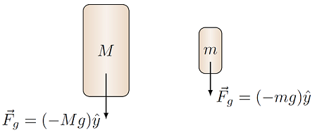
Fig. 21.8 Two falling objects, and the forces on them, near the surface of the Earth

Now what would the motion of the two masses look like if we filmed it with a high-speed camera? Neglecting air resistance, we would see the two move with exactly the same motion! Remember the cannonball and the feather movie back in Lesson 05. This is because the two masses have exactly the same acceleration.

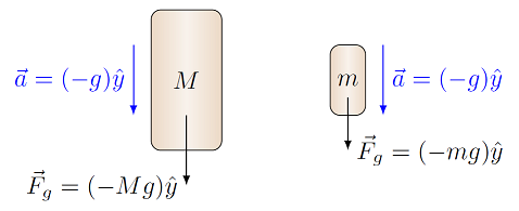
Fig. 21.9 Two falling objects, and their accelerations, near the surface of the Earth

Thus, we have found a quantity that is the same for all objects moving under the influence of gravity near the Earth. This is a measure of the Earth’s gravitational influence on other things close to it! This measure does not depend on the size of the object, just on the mass and radius of the Earth. If you use a large mass \(M\) to test this influence, while I use a small mass \(m\), we still get the same answer for their accelerations. These are the key points behind the gravitational field created by an object (here, the Earth):

1. The gravitational field created by the Earth is depends only on the properties of the Earth.

2. The gravitational field is the same, regardless of what mass you used to find its magnitude and direction. Here, the “test masses” were the two masses \(m\) and \(M\).

These are the basic properties of any kind of field. In Lesson 25, we will define an electric field, but again, these vectors will only depend what charge is creating them, not what is used to test them.

So how does this happen? Look back at the example in the previous section, and particularly at the algebraic expressions for the two force \({\vec F}_{12}\) and \({\vec F}_{13}\). You will notice that both of these forces are proportional to the mass \(m_1\) acted on by these forces. Said differently, this means that \({\vec F}_{12}\) is equal to \(m_1\) times some vector made of the “other pieces”, and the same is true for \({\vec F}_{13}\). We can factor out the mass affected by this net force. This is how we can define the gravitational field.

• Quantity: gravitational field

• Symbol: \({\vec g}\)

• Definition: Suppose a small mass \(m\) (known as a test mass) is placed at some distance away from a mass \(M\), which results in a gravitational force \(F_g\) on the test mass due to the mass \(M\). Then the gravitational field due to object \(M\) at the location of mass \(m\) is given by

\[ {\vec g} = \frac{{\vec F}_g}{m} \]

• SI Units: N/kg (equivalent to m/s\(^2\))

Suppose we want to find the gravitational field at a point \(P\), due to a mass \(m_j\), with the set-up as in the picture below.

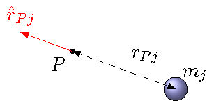
Fig. 21.10 Finding gravitational field due to mass \(m_j\)

Regardless of the size of the test mass \(m_P\) we place at \(P\), the gravitational field will be the gravitational force on \(m_P\), divided by the mass \(m_P\), so that

\[ {\vec g} = - \frac{(G m_P m_j / r^2 _{Pj})}{m_P} {\hat r}_{Pj} \]

If we simply this, we get the gravitational field due to a point mass \(m_j\) at a point \(P\) a distance \(r_{Pj}\) away from the mass \(m_j\) as

\[ {\vec g} = -\biggl( \frac{Gm_j}{r^2 _{Pj}} \biggr) {\hat r}_{Pj} \]

Notice this is just the same conceptual definition of the gravitational field we saw in Lesson 05. The only additional part is that we know can calculate the gravitational force \({\vec F}_g\) directly, and use it to find an equation for the gravitational field \({\vec g}\).

Problem

Between the red and the blue masses, which of them experiences the greater gravitational field magnitude due to the green mass?

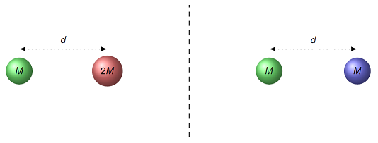
Fig. 21.11 Which of the two situations shown has a larger gravitational field due to the green mass?

Answer: The distances of both the red and blue masses from the green mass are the same, so the gravitational fields are the same as well.

Problem

Listed below are the radii and masses of various objects in the solar system; what would be the magnitude of the gravitational field for an astronaut standing on their surface?

Object	Radius (km)	Mass (kg)	Field (m/s\(^2\))
Mercury	2440	\(3.30 \times 10^{23}\)
Venus	6051	\(4.87 \times 10^{24}\)
Earth	6378	\(5.97 \times 10^{24}\)
Moon	1737	\(7.35 \times 10^{22}\)
Mars	3397	\(6.42 \times 10^{23}\)
Europa	1569	\(4.80 \times 10^{22}\)

Answer: Here is the completed table. Remember to convert each radius into meters!

Object	Radius (km)	Mass (kg)	Field (m/s\(^2\))
Mercury	2440	\(3.30 \times 10^{23}\)	3.70
Venus	6051	\(4.87 \times 10^{24}\)	8.87
Earth	6378	\(5.97 \times 10^{24}\)	9.79
Moon	1737	\(7.35 \times 10^{22}\)	1.62
Mars	3397	\(6.42 \times 10^{23}\)	3.71
Europa	1569	\(4.80 \times 10^{22}\)	1.30

Notice that we can use the definition of the gravitational field \({\vec g}\), in terms of the gravitational force, to simplify calculations. In the last section, for the example of the equilateral triangle, we solved for the net force on mass \(m_1\). Now that we have that, we can use the fact that

\[ {\vec g} = \frac{{\vec F}_1}{m_1} \]

to find the gravitational field at the location of \(m_1\). It doesn’t matter that there is an object at that point; we can think of this mass as the test mass we are using to find the field. Let’s do this calculation in two different ways, so you can see how it goes. First, we can use the unit vector form of \({\vec F}_1\):

\[ {\vec g} = \frac{(-1.366 \times 10^{-12} \textrm{ N}) {\hat x} + (-1.651 \times 10^{-11} \textrm{ N}) {\hat y}}{(2.00 \textrm{ kg})} \]

Dividing both components by the the mass \(m_1\), we get

\[ {\vec g} = (-6.830 \times 10^{-13} \textrm{ N/kg}) {\hat x} + (-8.255 \times 10^{-12} \textrm{ N/kg}) {\hat y} \]

Finding the magnitude and direction of this vector gives \(8.28 \times 10^{-12}\) N/kg at 275\(^\circ\) CCW from the \(+x\) axis. However, the attentive reader will notice something about this vector, leading to the second way we can find the gravitational field at the location of \(m_1\). This is the fact that this magnitude is simply the original force magnitude, divided by 2.00 kg; the direction is the same as the force itself! This works out because the mass is a positive number. We are scaling both components of the vector triangle by the same amount, so the hypotenuse changes by the same, and the direction is unaltered. This works for gravity, but be careful when we come back to this with electric fields (where the charges can be negative!).

Forces and fields

If you know one of either the gravitational field at a point, or the gravitational force on a charge at the same point, and are asked to find the other, don’t solve from scratch! It is much easier to use the definition of \({\vec g}\) to simplify the calculation.

Problem

For the equilateral triangle problem above, find the gravitational field at the location of mass \(m_3\).

Answer: \(7.20 \times 10^{-12}\) m/s\(^2\) at 161\(^\circ\) CCW from the \(+x\) axis

Problem

Two masses \(M\) and \(4M\) are fixed at a distance of \(3R\). Is there a location \(P\) on the line between the two masses such that the net gravitational field is zero? If so, give the distance from the mass \(M\) to this location, in terms of a multiple of \(R\). If not, explain why not.

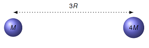
Fig. 21.12 Find the location between the two masses \(M\) and \(4M\) where the gravitational field is zero

Answer: The gravitational fields of each mass \(M\) and \(4M\) point towards that mass. Thus, at every point on the line between the two masses, their gravitational fields point in opposite directions. For them to cancel, their magnitudes must be the same. This happens when the distance between the location \(P\) and mass \(M\) is \(R\), which gives the distance between \(P\) and mass \(4M\) is \(2R\). Because the distance is twice as great to mass \(4M\), by the inverse square law, the magnitude of the gravitational field will be exactly the same as that from \(M\). This means there is a location closer to the smaller mass where the net gravitational field is the zero vector.

21.4. Summary

The gravitational force was one of the first examples of forces we worked with in Lesson 13 (solving force problems). However, at that point, we leaned heavily on the fact that the gravitational field is close to constant on the Earth’s surface, and used that fact to “define” the force of gravity on an object. We have now reached the point where we can define the gravitational force between any two point masses, not just the Earth and another (small) mass. If we were so inclined, we could built up the force between arbitrary objects by thinking of each of them as made of a collection of small masses. You may see something like that later in your academic career.

The gravitational force is the only truly long-range force in the Universe. We will see in Lesson 24 that Coulomb’s law for the electrostatic force has a similar form. But in practice, because there are both positive and negative charges, the electrostatic force tends to cancel out over large distances, and it does not have too much of an effect on astronomical scales. This is different than gravity, which is the force keeping the planets of the Solar System around the Sun, and the stars in our Milky Way galaxy in their spiral structure. Even the evolution of the Universe in time depends primarily on how gravity affects all the objects in it!

We also fleshed out the idea of a field, using the gravitational field as our first example. Remember to focus on the key ideas behind what a field is – a field measures the influence of an object on its surroundings. We say that falling objects have an acceleration of 9.81 m/s\(^2\) downward because that is the gravitational field near the surface of the Earth. This depends only on the mass and size of the Earth, not on the object’s mass. If we lived on another planet, we would remember another number for the magnitude, because the gravitational field would be different. However, this is also dependent on the physical properties of our environment. There are some spiders, for example, that use the electrostatic force for help getting from one plant to another. A physics class for intelligent spiders would memorize the size of the electric field at the Earth’s surface!

Fields are fundamental to our modern understanding of how physics works. Not only do they make the mathematics simpler, but they get at the heart of why objects have the properties that they do. Whenever you hear a physicist talk about a “quantum field theory”, they are thinking about using fields to describe the basic properties of matter. Fields are both powerful, and a natural way to describe the nature of the Universe.

After today’s class, you should be able to:

• Describe how the gravitational force between two objects changes as their masses or distance change by some proportion.

• Calculate the gravitational force between two objects.

• Define gravitational field, and state its SI units.

• Calculate the gravitational field at some distance from a mass.

20. Conservation of energy 22. Gravitational potential energy