.ipynb .pdf

Binder

Contents

12. Solving force problems

12.1. Overview

We have started with the basic definitions of momentum, and used it in Newton’s laws of motion to consider the collision of objects. Hopefully, this gives you a sense of some of the important aspects of forces – forces are due to an interaction between two objects, and over a time interval will change the momentum of each of the objects.

However, there are many more forces that we have not considered. I am sure that, after a moment’s thought, you can make a long list of forces acting on objects. A few forces we will discuss over the coming lessons are friction, buoyancy, and gravity. Because these forces can have different properties, it is important to develop a standard way of combining these forces together to find the motion of the object they act on. This recipe is what is covered in this lesson. In particular, we will look at free body diagrams as a visual way of finding the correct Newton’s 2nd law equation of a particular system.

Newton’s second law is a method

There is a standard method for solving force problems, but there is not a standard equation. Every time you have forces involved in a situation, you should start with a free body diagram and Newton’s 2nd law. But the equation you derive from Newton’s 2nd law will be different in each case! This is because the forces may be different, or the directions they act in may change. You will have to think through what is affecting the system, but always using the force equations to do so. This lesson will help to build that intuition within you.

Here are the objectives for this lesson:

• Describe how to draw the free body diagram for an object with one or more forces acting on it.

• Calculate the acceleration or final velocity of an object after it experiences a force over a given time interval.

• Given the gravitational field at an object’s location, state the gravitational force on that object.

• State the direction of the tension force acting on an object.

• Define the normal force.

• Describe the difference between the static frictional force and the kinetic frictional force.

• State the relationship between the frictional force and the normal force.

• State the maximum value of the static frictional force.

• Given an object moving along a surface with friction, calculate the acceleration of the object.

12.2. Free body diagrams and Newton’s 2nd law

One of the convenient facts about the Universe is that you can solve for the overall motion of a complicated system by considering only a few pieces of information. We have seen this before in previous lessons – for example, how a system of multiple objects can be thought of as a single point, moving along with the center of mass velocity of the system. We will build on this when considering forces.

Since we can simplify things quite a bit, it makes sense to represent the situation for a system by drawing only those pieces of information that are required. This leads to the idea of a free body diagram. A free body diagram (abbreviated FBD) is a picture of the forces acting on a system, a way of succinctly summarizing the forces acting on a system, a single object, or at a single point. We will use these as a thinking aid when solving the equations of Newton’s 2nd law.

Because we are eliminating any non-essential information in a free body diagram, only the force vectors, and the angles needed to find their components, will be included. This allows for the possibility that a lot of forces are acting on the system at once.

Guidelines for drawing an FBD

1. Draw the object as a dot; if desired, draw \(x\) and \(y\) axes with the object at the origin

2. Draw all forces (not their components!) as arrows

   • Forces always point away from the object

   • Draw appropriate angles for forces next to the dot

   • Be careful of direction of forces

   • Label forces and angles symbolically (no numbers)

3. Do not include other vectors

   • No acceleration

   • No velocity

   • No net force

4. In Lesson 19 (work and energy), we will add the displacement vector to FBDs, to help solve for work

Below is an example of a physical situation, and its corresponding FBD.

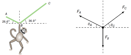
Fig. 12.1 A monkey hanging off of a vine, and the free body diagram at the location of its hand

Here, a monkey hanging off of a vine. Obviously, the force of gravity is acting downward on the monkey, so that means there is a like downward force on the vine at point \(B\). This bends the vine, so at the monkey’s hand, two tension forces are acting, one each to the left and right. Thus, the hand is where multiple forces are acting at once. The monkey will remain stationary only if these three forces add up to zero as vectors.

This is represented in the free body diagram to the right of the illustration. Because we are interested in maintaining equilibrium, the FBD is drawn at the point where the monkey’s hand is grabbing the vine. The three forces acting at that point are then represented as vectors, pointing away from the dot indicating the position of the hand. This FBD shows all the information needed to write down the Newton’s 2nd law equations for that position.

Next, we will formally introduce the two forces from the free body diagram above – the tension force, and the force of gravity.

12.3. The tension force

If something like a rope or string (or a vine!) is attached to an object, and then pulled on, that object will experience a tension force. This force will act at the point of contact between the rope and the object, and point in the direction along the rope at this contact point. So really, this is a type of applied force, and its magnitude can change, depending on how hard the rope is pulled on. You can imagine a tug-of-war, where the winner is determined by who can pull hardest; this can change, depending on who is working the rope.

This means that there is no set value or equation for the tension force. Assuming the rope is strong enough, it can be any magnitude. This will usually be a given number, but sometimes it may be something you are solving for.

Problem

Two crewmen pull a raft through a canal lock, with their forces shown in the figure below. One crewman pulls with a force of 130. N at an angle of 34.0\(^\circ\) relative to the forward direction of the raft. The second crewman, on the opposite side of the lock, pulls at an angle of 45.0\(^\circ\).

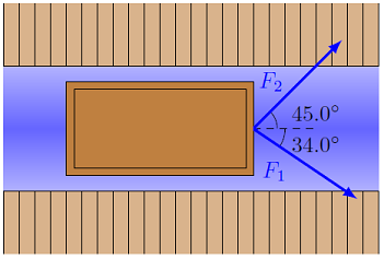
Fig. 12.2 Raft pulled along a canal

1. With what magnitude of force \(F_2\) (in N) should the second crewman pull so that the net force of the two crewmen is only in the forward direction (if the angle is kept the same)?

2. What is the magnitude of the net force (in N) on the raft (assuming it is being pulled straight forward)?

Answers: 103 N; 181 N

Problem

The first crewman is a bit of a jokester, and likes to change the angle at which he pulls the raft. Help the second crewman by creating a vPython function secondAngle(). This function should return the angle (in degrees) that the second crewman should pull the raft, so that the net force on the raft is only in the forward direction, down the canal. The arguments of the function should be the scalars F1 and F2, for the magnitudes of the two crewmen’s given forces \(F_1\) and \(F_2\), and the angle (in degrees) Q1 that the first crewman pulls the raft.

You will need to use the inverse trigonometric functions in vPython. The functions asin(), acos(), and atan() correspond to the functions \(\sin^{-1}(), \cos^{-1}()\), and \(\tan^{-1}()\), respectively. These functions will return values in radians, not degrees, so you need to convert back!

Note: There are certain values of these arguments where there is no angle at which the second crewman to pull, so that the net force is in the right direction! Your function should print out Impossible situation if this is true, and return the value -1.

Answer: Here is an example function.

def secondAngle(F1, F2, Q1):

    # Find the x and y components of the
    # force due to the first crewman;
    # remember to convert first to radians!
    
    F1x = F1 * cos(radians(Q1))
    F1y = F1 * sin(radians(Q1))
    
    # If F1y is greater than the magnitude
    # F2, then the situation is impossible
    
    if F1y > F2:
        print('Impossible situation')
        return -1
        
    # If the situation is possible, then
    # the y components of the two forces
    # must be equal and opposite, so that
    # F2 sin(Q2) = F1y. This can be solved
    # using the inverse sine function, or
    # asin()

    return degrees(asin(F1y / F2))

12.4. The gravitational force

Before we talk about how to calculate the gravitational force \({\vec F}_g\), it is important to talk first about terminology. On Earth, we frequently use the terms “mass” and “weight” interchangeably, and this is not too far off. Since the gravitational field is roughly constant everywhere on the surface of the Earth, then the mass and weight of an object will always be proportional.

But there is an important conceptual distinction that this glosses over. When we say mass, we are referring to the amount of “stuff” an object has. This is a fixed property, as long as the object is not split into pieces. Another way to say this is that mass is the measure of inertia – as we saw with Newton’s 2nd law, for the same net force, an object with larger mass will have a smaller resulting acceleration. More massive objects are harder to move.

This is different that the weight of an object. Weight is the gravitational force on an object. So, unlike mass (which is a scalar), weight is a vector quantity, with both magnitude and direction. On the Earth’s surface, the weight is always acting towards the center of the Earth, which is why we usually don’t mention it when state our weight. As we will see shortly, it depends on the object’s mass, but it also depends on the gravitational field. Since weight is a force, we will use the symbol \({\vec F}_g\) for it. I will use “weight” and “gravitational force” as synonyms, so remember that weight is a vector, not a scalar.

Back in Lesson 05 (acceleration and free fall), the gravitational field \({\vec g}\) was described as the strength of the gravitational influence of an object on everything around it. Now that we are talking about forces, we can be more explicit in what this means. Once you know what \({\vec g}\) is at the location of an object with mass \(m\), then the gravitational force \({\vec F}_g\) on that object is given by

\[ {\vec F}_g = m {\vec g} \]

Thus, this now explains something else said in Lesson 05: if gravity is the only force acting on the object, then its acceleration is the same as the gravitational field. You can see this by using Newton’s 2nd law. Since the mass \(m\) is in free fall, then the sum of the force is just \({\vec F}_g\):

\[ \sum {\vec F} = m {\vec g} \]

Newton’s 2nd law says that the sum of the forces on \(m\) is

\[ \sum {\vec F} = m {\vec a} \]

so we can see that the object’s acceleration \({\vec a} = {\vec g}\).

However, in general, there are multiple forces acting on an object, so \({\vec g}\) will not be the object’s acceleration. This is why we describe it as a measure of gravitational influence. In Lesson 21 (gravitational force), we will see how to calculate \({\vec g}\) in general. This will include not only how to find \({\vec g}\) near the surface of the Earth, but also when there are multiple sizable objects present.

Problem

One way to lose weight is to go to another planet! Suppose an 80.0 kg person weighs themself on the Earth, then travels to the Moon, where \(g = 1.63\) m/s\(^2\), and they weigh themselves again. How much weight (in N) did they “lose” by going to the Moon?

Answer: 654 N

Problem

Write a Python procedure surfaceWeight() that prints out the values of the weights for an object on various planets and satellites in the Solar System; remember to include the appropriate units. The procedure takes as an argument mass the mass of the object. Use the gravitational field magnitudes listed in the table below.

Location	Field (m/s^2)
Mercury	3.70
Venus	8.87
Mars	3.71
Europa	1.62
Pluto	0.620

Answer: One possible procedure is given below.

def surfaceWeight(mass):

    # Define gravitational field magnitudes
    # (all in m/s ** 2)

    gMer = 3.70
    gVen = 8.87
    gMars = 3.71
    gEur = 1.62
    gPlu = 0.620

    # Print out weight magnitudes

    print('Weight on Mercury: ' + str(gMer * mass) + ' N')
    print('Weight on Venus: ' + str(gVen * mass) + ' N')
    print('Weight on Mars: ' + str(gMars * mass) + ' N')
    print('Weight on Europa: ' + str(gEur * mass) + ' N')
    print('Weight on Pluto: ' + str(gPlu * mass) + ' N')

12.5. Example: Hanging ball

Let’s work through an example problem and see how to find the magnitude of two tension forces acting on an object. Here, you will see how to draw an FBD for the problem, then write down the appropriate force equations, using Newton’s 2nd law.

Here is the situation to consider. A ball of mass 100. g is attached to both the wall and ceiling, as shown. String 1 is completely horizontal and string 2 makes an angle \(\theta\) of 60.0\(^\circ\) with the ceiling. We are going to calculate the sizes \(F_{T1}\) and \(F_{T2}\) of the tension forces acting on the ball. The physical situation is shown in the picture below.

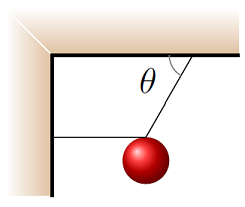
Fig. 12.3 A ball held in place by two strings

The tension \({\vec F}_{T1}\) is acting on the ball along string 1, and similarly for \({\vec F}_{T2}\). Notice that there is also a gravitational force acting on the ball, which is why the ball’s mass will be important.

Our first step will be to draw the FBD for the ball. Why are we choosing the ball as the system to consider? Well, this is the object on which all the forces of interest are acting on. By Newton’s zeroth law (see Lesson 10), the forces acting directly on the ball are the two tension forces and the ball’s weight. We know enough to calculate the weight, and we want to find the tensions, so this is everything we want! Now, let’s draw the FBD for the ball. Remember to draw the arrows away from the dot representing the ball, in the same direction as the actual forces. This gives the FBD below for the ball.

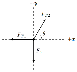
Fig. 12.4 The FBD for the hanging ball

Notice I have moved the angle, so that it is next to the origin of the diagram. The angle here is the same as the angle shown in the physical diagram, because of alternate interior angles.

Now that we have our FBD, we can use it to write down the Newton’s 2nd law equations for this situation. If I write this down as a vector equation, I get

\[ \sum {\vec F}_{ball} = {\vec F}_{T1} + {\vec F}_{T2} + {\vec F}_g = m_{ball} {\vec a} \]

This is a vector equation, so the directions are “inside” the vectors. Thus, there are no minus signs just yet; these will come in when we write down the components of each vector, which will be our next step. But first, since the ball is not moving, it is definitely not acceleration, so we can say \({\vec a} = {\vec 0}\).

The next step is to find the components of each force, in terms of their magnitudes. This will be useful in getting equations to solve for each tension magnitude. We are still doing algebra here, so only symbols, no numbers just yet. Two of the forces are along the coordinate axes, so they are simple:

\[ {\vec F}_{T1} = (-F_{T1}) {\hat x} \qquad {\vec F}_g = (-F_g) {\hat y} \]

As always, the vector is written with the arrow sign, while the magnitude is written without. The directions of each force component is shown by the negative signs and the unit vectors \({\hat x}, {\hat y}\). For the last vector \({\vec F}_{T2}\), we need to find the \(x\) and \(y\) components, so we draw a vector diagram to help.

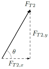
Fig. 12.5 Vector diagram for tension \({\vec F}_{T2}\)

This gives that the second tension force vector is

\[ {\vec F}_{T2} = (F_{T2} \cos \theta) {\hat x} + (F_{T2} \sin \theta) {\hat y} \]

These are now combined into Newton’s second law. We take the vector version of it, given above, and write down separately the \(x\) and \(y\) components of the equation. In Lesson 13 (scalar product), we will see how to do this more formally. For now, though, this gives

\[ F_{ball, x} = -F_{T1} + F_{T2} \cos \theta = m_{ball} a_x = 0 \]

and

\[ F_{ball, y} = F_{T2} \sin \theta - F_g = m_{ball} a_y = 0 \]

Remember these net force components are equal to zero, since \({\vec a} = {\vec 0}\). We now have two equations we can solve for the magnitude \(F_{T1}\) and \(F_{T2}\), in terms of the angle \(\theta\) and the gravitational force \(F_g\). But we have to be careful how we solve these! The \(x\) equation has both unknowns in it, so we need to solve the \(y\) equation first, resulting in

\[ F_{T2} = \frac{F_g}{\sin \theta} = \frac{m_{ball} g}{\sin \theta} \]

In the second step, we used the fact that the magnitude \(F_g\) of the ball’s weight is \(m_{ball} g\). This equation can be substituted into the \(x\) equation to find \(F_{T1}\).

\[ F_{T1} = F_{T2} \cos \theta = \frac{m_{ball} g \cos \theta}{\sin \theta} = \frac{m_{ball} g}{\tan \theta} \]

The last step here uses the definition of \(\tan \theta\) as the ratio of \(\sin \theta\) and \(\cos \theta\). Plugging in the givens into these equations gives

\[ F_{T1} = \frac{(0.100 \textrm{ kg})(9.81 \textrm{m/s}^2)}{\tan 60.0^\circ} = 0.566 \textrm{ N} \qquad F_{T2} = \frac{(0.100 \textrm{ kg})(9.81 \textrm{m/s}^2)}{\sin 60.0^\circ} = 1.13 \textrm{ N} \]

Since \(F_{T1} = F_{T2} \cos \theta\), and \(\cos 60.0^\circ = 0.500\), then \(F_{T1}\) is exactly half the size of \(F_{T2}\). This would not be true for any other angle \(\theta\).

Problem

A 124 N stop light hangs at rest from two cables as shown below, where \(\theta_1=30.0^\circ\) and \(\theta_2=50.0^\circ\). Solve for the magnitudes of the tensions \(F_{T1}\) (left rope) and \(F_{T2}\) in the two ropes (in N). Hint: The Newton’s 2nd law equations will have both unknown magnitudes in both \(x\) and \(y\) equations, so you will have to use the techniques of simultaneous equations (as I did in the example above) to find these values.

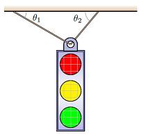
Fig. 12.6 A hanging stoplight

Answers: \(F_{T1} = 80.9\) N; \(F_{T2} = 109\) N

Problem

As an employee of the City of Newport, your job is to hang up streetlights. However, you are concerned that the ropes used are not strong enough when the streetlights are hung at certain angles.

1. Based on your work for the previous problem, write down equations for the tension values \(F_{T1}\) and \(F_{T2}\) in each rope, using the variables \(m\) (streetlight mass), and \(\theta_1, \theta_2\) (the two rope angles). Hint: Your equations will simplify quite a bit if you use the trigonometric identity \(\sin (\theta_1 + \theta_2) = \sin \theta_1 \cos \theta_2 + \cos \theta_1 \sin \theta_2\).

2. Suppose that \(\theta_1 > \theta_2\). Which tension value will then be the larger one?

3. Write a vPython procedure checkTension() that checks whether the tension values in the ropes exceeds the maximum safety value. The arguments of the procedure should be m for the streetlight mass, Q1 and Q2 for the angles \(\theta_1\) and \(\theta_2\), respectively, and F_MAX for the maximum safe value of the rope tension magnitude. If the situation is safe, have the procedure print out OK; otherwise, the procedure should print out Unsafe situation.

Answers: The equations for the two tension magnitudes are given by \(F_{T1} = mg \cos \theta_2 / \sin(\theta_1 + \theta_2)\) and \(F_{T2} = mg \cos \theta_1 / \sin(\theta_1 + \theta_2)\). Since \(\theta_1 > \theta_2\) implies that \(\cos \theta_1 < \cos \theta_2\), then \(F_{T1}\) would be the larger magnitude. This makes physical sense, because whichever rope has the larger angle will be supporting more of the streetlight’s weight.

Here is a possible procedure for checking whether the situation is safe.

def checkTension(m, Q1, Q2, F_MAX):
    
    # Define grav field magnitude
    
    g = 9.81          # in m/s^2
    
    # Check which angle is larger,
    # to know which tension value
    # is larger
    
    if Q1 > Q2:       # check F_T1
    
        F_T1 = (m * g * cos(Q2)) / sin(Q1 + Q2)
        if F_T1 > F_MAX:
            print('Unsafe situation')
        else:
            print('OK')
            
    else:             # Q1 < Q2, check F_T2
    
        F_T2 = (m * g * cos(Q1)) / sin(Q1 + Q2)
        if F_T2 > F_MAX:
            print('Unsafe situation')
        else:
            print('OK')

12.6. Normal force

The best way to think about the normal force is that it is the force that prevents one object from passing through another. When you sit on a chair, or lean against a wall, these objects exert a normal force on you, so you do not fall through the chair or wall. The normal force is known as a constraint force, since it constrains objects from occupying the same location!

Notice that the normal force can change, depending on the situation. If you think of yourself leaning against the wall, with your feet still on the floor, both the wall and floor exert normal forces on you. If you change your angle relative to the horizontal (your “lean”), then the sizes of the two normal forces will shift. When you are almost vertical, the floor acts on you with the larger normal force; if you move your feet away from the wall, the angle with the horizontal will decrease, and the wall exerts a normal force with increasing size. The important point is that these forces constrain you, so that you don’t accelerate through the wall or floor!

Each of these forces prevent you from passing through the floor or wall, so they must be perpendicular to these surfaces – you don’t start sliding sideways, just because you are standing on the floor! Similarly with the wall, where you may slide down the wall, but that is due to gravity, not the force of the wall on you. These forces also point away from the surface (floor or wall).

Properties of the normal force

The normal force is a force that a surface exerts on an object. The normal force on the object always points perpendicular to (and away from) the surface. The magnitude of the normal force is whatever amount is required to prevent the object from accelerating through the surface. There is no direct relationship between the magnitudes of the normal force and the weight!

Problem

What is the correct direction for the normal force given that the object is resting on an inclined surface, as shown below?

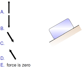
Fig. 12.7 Find the correct direction for the normal force on a block sitting on a ramp

Answer: The normal force points up and to the left.

Problem

What is the correct direction for the normal force on an object pressed against a horizontal surface?

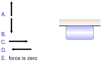
Fig. 12.8 Find the correct direction for the normal force on the block on the ceiling

Answer: The normal force points downward.

Problem

What is the correct direction for the normal force given that the object is hanging by a string above a horizontal surface?

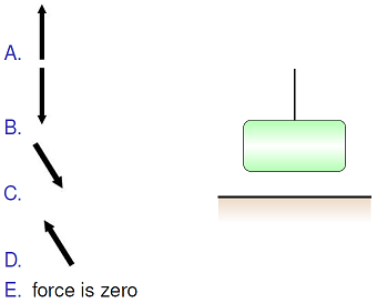
Fig. 12.9 Find the correct direction for the normal force on the hanging block

Answer: The block is not on a surface, so there is no normal force.

Let’s go through an example, to see how this works in a calculation. A 1.50 kg object is pushed up a frictionless vertical wall with a force \(F\) at an angle of 35.0\(^\circ\) above the horizontal. Starting from rest, the block is moving with an upward velocity of 11.0 m/s after two seconds. We will find the magnitude of the applied force \(F\), and the magnitude of the normal force \(F_N\).

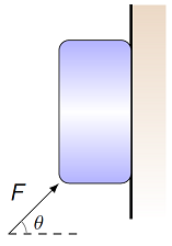
Fig. 12.10 A block pushed up the wall

First, we draw an FBD for this situation. Notice that, since the normal force is away from the surface and perpendicular to it, then \({\vec F}_N\) points to the left.

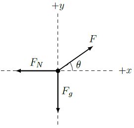
Fig. 12.11 The FBD for the block pushed up the wall

Writing down the sum of the forces acting on the wall, we get

\[ \sum {\vec F} = {\vec F}_N + {\vec F} + {\vec F}_g \]

Now, we find the force vector component equations along each coordinate axis. This gives

\[ \sum F_x = -F_N + F_x = ma_x\qquad \sum F_y = \sum F_y = F_y - F_g = ma_y \]

Here, \(F_x\) and \(F_y\) are the \(x\) and \(y\) components of the applied force \({\vec F}\). The block is accelerating upwards, since its velocity is increasing in that direction. However, horizontally the block is not moving, so \(a_x = 0\). This means we can solve first for the relation between the normal force magnitude \(F_N\) and the size of the applied force \(F\).

\[ -F_N + F_x = 0 \Rightarrow -F_N + F \cos \theta = 0 \Rightarrow F_N = F \cos \theta \]

This makes sense – the normal force is canceling out the piece of the applied force that is directly into the wall; it is not affected by the vertical component of the applied force. This latter part will change the acceleration in the \(y\) direction, so let’s look at that now. By definition,

\[ a_y = \frac{\Delta v_y}{\Delta t} \]

and with \(v_{i, y} = 0\), then the force equation in the \(y\) direction becomes

\[ F \sin \theta - mg = \frac{mv_{f, y}}{t} \]

Solving this for the applied force magnitude \(F\) gives

\[ F = \frac{m(g + v_{f, y} / t)}{\sin \theta} \]

and a value of \(F = 40.0\) N. Using this in the equation solved above for the normal force gives \(F_N = 32.8\) N.

Problem

A 7.85 kN telephone pole is shown in the figure. Assume that the normal force on the telephone pole is vertically upwards with a value of 21.0 kN, and the angles are \(\theta = 30.0^\circ\) and \(\phi = 40.0^\circ\).

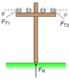
Fig. 12.12 A telephone pole held in place with two cables

1. What is the magnitude of the tension \(F_{T1}\) (in kN)?

2. What is the magnitude of the tension \(F_{T2}\) (in kN)?

Hint: The Newton’s 2nd law equations will have both unknown magnitudes in both \(x\) and \(y\) equations, so you will have to use the techniques of simultaneous equations to find these values.

Answers: \(F_{T1} = 1.07\) kN; \(F_{T2} = 1.21\) kN

12.7. Friction

12.7.1. The study of friction

If you have some discomfort with Newton’s first law of motion, it’s probably because of the widespread presence of frictional forces in our everyday lives. Whenever we roll a ball along a table, the ball will eventually stop, not because that is the “natural” motion of all objects, but because of friction between the ball and the table. This was one of the difficult mental leaps that had to be made to go from the thoughts of Aristotle and the ancient Greeks, to the modern viewpoint on physics: motion stops because there are forces present that cause this stop, not because the “natural state” of an object is always at rest. This flip between viewpoints allows us to describe in detail the forces that cause motion to change, rather than throwing up our hands and saying it’s the way things are.

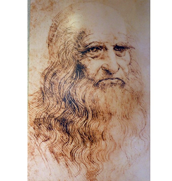
Fig. 12.13 A self-portrait of Leonardo da Vinci from his notebooks

This leads us into the specific force of friction as our next topic. Leonardo da Vinci was one of the first people to systematically examine the size of the frictional force. In a series of experiments, he showed that friction does not depend on the contact area between the two surfaces, and that increasing the load on an object will increase the frictional force proportionally. However, although his discoveries were written into his notebooks, these were not publicly known until hundreds of years later.

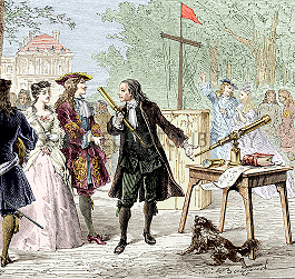
Fig. 12.14 Guillaume Amontons showing the Dauphin of France his method to transmit message by optical telegraphy

da Vinci’s laws of friction were rediscovered by the French instrument maker and physicist Guillaume Amontons around 1700, and hence are often called “Amontons’ laws”. These rules were verified by Charles-Augustin de Coulomb (whom we will see later with the electrostatic force in Lesson 24) about eight decades later.

The frictional force is a complicated area of study, and researchers are continuing to look into its properties. This is because, not only is it interesting, but it has obvious industrial and engineering applications. We will examine only a simple model of friction here.

12.7.2. Two types of friction

Suppose you are rearranging the furniture in your living room, and decide you want to move your couch. You give it a push to slide it along the carpet in the room. To make things definite, let’s make it a couch with a weight of 2.00 kN, and you start out by applying a force of 200. N to the couch. It doesn’t move, so you push harder with 400. N. It still doesn’t move, so you push with 600. N. Still doesn’t move. You activate those honed muscles of yours and push with 800. N, which is finally enough to get the couch to move. Not only does it move, but it starts accelerating across the living room! So, you push with only 600. N, and (unlike before), the couch now moves at a constant velocity.

I’m sure you can think of some situation like this, where you have to apply a force to get something to start moving. Once you do get it moving, you need less force to keep it moving. This shows that there are two separate types of frictional force. The static frictional force acts on an object when it is stationary relative to the surface it is sitting on. Notice that they may be moving together – think of a crate in the flatbed of a pickup truck, for example. The kinetic frictional force acts on an object moving relative to the surface it is on. This may be due to the object moving on a stationary surface, or the other way around. The magnitude of the kinetic frictional force is usally less than that of the static frictional force.

Once the couch in the example above starts moving, then only the kinetic frictional force is acting on it. Before that, however, your applied force is opposed by the static frictional force. Note how the type of frictional force changed! As you increased the applied force, the static frictional force matches it, at least up to a point. Beyond that maximum, though, friction was not strong enough to prevent the couch from moving, and now the kinetic friction was involved.

As mentioned above, da Vinci, Amontons, Coulomb, and others started a detailed study of the properties of the friction force. Their model of friction, described in this lesson, has two basic properties.

Properties of the frictional force

1. The direction of the frictional force \({\vec F}_{fr}\) is always opposing the motion of an object, or the potential motion, if the object is at rest.

2. The magnitude \(F_{fr}\) of the frictional force on an object on a surface is proportional to the normal force due to the surface, acting on the object. The constant of proportionality is known as the coefficient of friction, and given by the symbol \(mu\) (“mu”).

Let’s talk about these in more detail, starting with the direction. Think again to the example mentioned earlier of a crate in a flatbed truck. As the truck drives along, if the flatbed’s surface were completely smooth, the crate would have no horizontal force on it, and it would slide backwards. To keep the crate in place, the static frictional force acts opposite to this motion, in the direction the truck is moving. This is what I mean by opposing the potential motion of the object. Thus, it is actually the frictional force moving the crate forward! Think about that the next time you go for a walk.

For the magnitude, since the force of friction is always proportional to the normal force, then it makes sense to look at the ratio of the frictional and normal forces; this will be the constant \(\mu\) mentioned above. Thus, the coefficient \(\mu\) is the ratio of the two magnitudes, or

\[ \mu = \frac{F_{fr}}{F_N} \]

Notice that, since \(\mu\) is the ratio of two forces, it has no units! This constant is roughly the same for a given type of friction (static or kinetic) with any pair of surfaces, e.g. rubber on carpet, for someone walking in their house with shoes on. There will be a coefficient of static friction \(\mu_s\) and a coefficient of kinetic friction \(\mu_k\) for each such surface pair. These coefficients must be measured experimentally, by going into the lab and moving the two surfaces against each other.

Let’s now get specific about the relationship between the normal and friction forces. Remember the example we had above, with the couch. Specifically, the static frictional force would change, since you altered your applied force. Thus, the force of static friction will actually have a range of values, up to some maximum static frictional force. To show this, the magnitude of \(F_{fr, s}\) is given by an inequality; the static frictional force is limited by its largest magnitude. Mathematically, this is

\[ F_{fr, s} \le \mu_s F_N \]

where, as before, \(F_{fr, s}\) is the force of static friction, \(\mu_s\) is the coefficient of static friction, and \(F_N\) is the normal force. On the other hand, the kinetic frictional force is constant, so it is a straight equality:

\[ F_{fr, k} = \mu_k F_N \]

where \(F_k\) is the force of kinetic friction, and \(\mu_k\) is the coefficient of kinetic friction.

The PhET application linked below allows you to play around with the force of friction, especially if you select the “Friction” portion of the app.

Use the “Friction” part of the PhET to answer the following questions.

Problem

Using the default values in the PhET, what is the coefficient of static friction between the crate and the ground? What is the coefficient of kinetic friction? Does it matter if you change the object you are pushing, or add mass on top of it?

Answer: The crate has a mass of 50 kg, so the gravitational force on it is 490. N. By steadily increasing the applied force when the crate is at rest, you find that the maximum static frictional force is 125 N. This gives \(\mu_s\) to be around 0.26. Once the crate is moving, there is a kinetic frictional force of 94 N, giving \(\mu_k\) to be around 0.19. These coefficients appear to be the same for all objects, which you can test by finding the necessary force to get each object to start moving.

Problem

Find the value of the unknown mass for the gift-wrapped box.

Answer: By increasing the applied force from zero, while the box is at rest, the maximum static frictional force is 125 N. When the box is moving, there is a constant kinetic frictional force of 94 N. Using the same coefficients of friction obtained in the last problem, this suggests the box has a mass of 50 kg. You can confirm this by adding objects with known mass, and verifying the frictional force changes as expected.

As another demonstration of the frictional force, let’s make a table of the applied forces on the couch. We assume that your applied force and the force of friction are the only horizontal forces.

Problem

Let the coefficient of static friction \(\mu_s\) be 0.375, and the coefficient of kinetic friction \(\mu_k\) be 0.250. Remember that the couch has a weight of 2.00 kN. If the living room floor is flat, use this to calculate the values of the maximum static frictional force, and the kinetic frictional force, and fill in the values of the frictional force in the table below.

\(F_{app}\) (N)	\(F_{fr}\) (N)
200.
400.
600.
800.

Answer: For this problem, you first need to find the normal force of the floor acting on the couch. Since the floor is flat, the magnitude of the normal force is equal to the value of the couch’s weight, or 2.00 kN. This means the maximum magnitude of the static frictional force is \(\mu_s F_N = (0.375)(2000 \textrm{ N}) = 750.\) N, while the constant value of the kinetic frictional force is \(\mu_k F_N = (0.250)(2000 \textrm{ N}) = 500.\) N. Then, the completed table of frictional forces should look like the one given below.

\(F_{app}\) (N)	\(F_{fr}\) (N)
200.	200.
400.	400.
600.	600.
800.	500.

Problem

After the couch starts moving, and you apply a force of 600. N on it, what is the frictional force value between the floor and the couch?

Answer: Once the couch is moving, the frictional force is kinetic, so the force of friction has a magnitude of 500. N.

12.8. An example: Multiple forces

Now that we have a model of the frictional force, let’s see how it interacts with some of the other forces we have dealt with. I will work through the following example. A block with a mass of 5.00 kg is moving because of a 20.0 N applied acting at an angle of 15.0\(^\circ\) below the horizontal. The coefficient of kinetic friction between the block and the horizontal surface is 0.200. Determine the horizontal acceleration (magnitude in m/s\(^2\)) of the block.

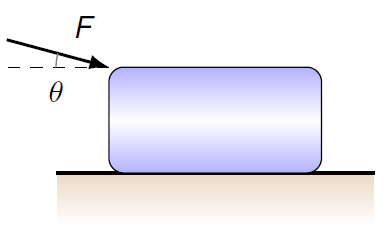
Fig. 12.15 Sliding a block

As always, the first step should be to draw a FBD for the block. This will include not only the frictional force, but also the gravitational, normal, and applied forces. The FBD of the block is shown below.

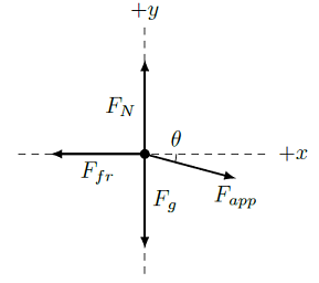
Fig. 12.16 FBD for block sliding on floor

You might think we only need to find the horizontal forces on the block, but since the friction force depends on the normal force, we need to solve for the vertical forces as well. In addition, the downward acting applied force will change the normal force, so we need to look out for that. If we write down the net force on the block, we have

\[ \sum {\vec F} = {\vec F}_{fr} + {\vec F}_N + {\vec F}_{app} + {\vec F}_g \]

Taking the \(x\) and \(y\) components, then

\[ \sum F_x = -F_{fr} + F_{app} \cos \theta = ma_x \]

and

\[ \sum F_y = F_N - F_{app} \sin \theta - F_g = ma_y \]

We solve first for the normal force magnitude \(F_N\), using the fact that \(a_y = 0\) (the block is not accelerating vertically). Then,

\[ F_N = F_{app} \sin \theta + mg \]

We know the block is moving, so the frictional force is kinetic; substituting the normal force into the kinetic friction force equation, the \(x\) force equation becomes

\[ -\mu_k (F_{app} \sin \theta + mg) + F_{app} \cos \theta = ma_x \]

With a little rearranging, this gives the size \(a_x\) of the acceleration to be

\[ a_x = -\mu_k g + \frac{F_{app} (\cos \theta - \mu_k \sin \theta)}{m} \]

Plugging in the given values results in an acceleration of 1.69 m/s\(^2\) to the right.

Problem

A 500. N crate starts at rest on the concrete floor of a warehouse. You exert a horizontal applied force of 350. N. The coefficient of static friction is 0.735, and the coefficient of kinetic friction is 0.580.

1. What is the acceleration of the crate?

2. What force is necessary to get the crate moving?

Answers: 0.00 m/s\(^2\); 368 N

Problem

An applied force \(F_{app}\) exerted horizontally starts to act on a 125 N block initially at rest. Below is shown a graph of the frictional force \(F_{fr}\) on the block from the floor, as a function of the applied force as it increases in size from zero newtons. Use this graph to find the values of the coefficients of static and kinetic friction.

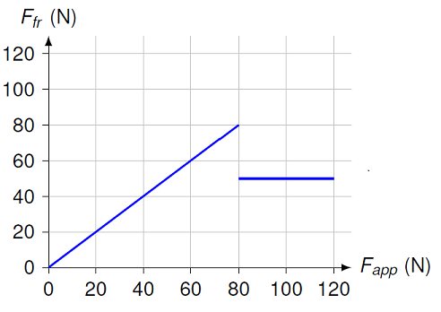
Fig. 12.17 Frictional force vs. applied force graph for sliding block

Answers: \(\mu_s = 0.640\), \(\mu_k = 0.400\)

Problem

A NAPSter, crazed by the latest victory of the football team, uses a force \({\vec F_{app}}\) of magnitude 90.0 N to push a 4.00 kg block across the ceiling of their room, as shown below. The coefficient of kinetic friction between the block and the ceiling’s surface is 0.400. Find the magnitude of the block’s acceleration (in m/s\(^2\)).

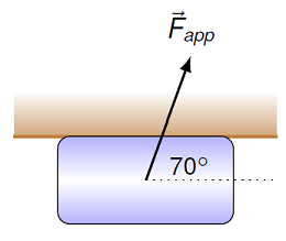
Fig. 12.18 Sliding a block on the ceiling

Answer: 3.16 m/s\(^2\)

12.9. Summary

We are now beginning to use force methods to solve problems. This lesson introduced this technique, and started with the tension, gravitational, normal, and frictional forces as examples to see how it works. Over the course of the next few lessons, we will add on additional forces, thus allowing us to look at more complicated situations. The basic ideas from this lesson will hold: the basic technique is to start with an FBD, and derive the appropriate force equations using Newton’s 2nd law. This should be your standard practice!

After this lesson, you should be able to:

• Draw the FBD of a system for any given physical situation

• Using the FBD, write down the appropriate Newton’s 2nd law equations

• Find the gravitational force on an object in a gravitational field

• Solve for the normal force acting on an object

• Describe what type of friction is appropriate for a given situation

• Explain how much static frictional force is present when other forces are applied to a stationary object

• Use a knowledge of forces and Newton’s second law to write down the appropriate mathematical relationship between the forces and the object’s acceleration.

11. Center of mass and collisions 13. Scalar product