26. Magnetic fields and forces
26.1. Overview
Link to the program in this lesson:
After the gravitational field, magnetic fields are probably the next most common example of a field in everyday life. I am sure you have played around at least once with bar magnets, and seen how the various poles of the magnets attract or repel. You may also have used a compass to navigate around, emulating sailors who have done this for centuries. In fact, the Chinese have been using compasses for that purpose for over a thousand years. Before that, they used the magnetic properties of lodestones for divination; it is not too surprising that a mystical purpose was given to stones that naturally seek to align with the Earth’s magnetic field! In today’s technology, magnets run the gamut from the speakers in your headphones, to the “M” in “MRI” when you go to the doctor’s office.
In this lesson, we will explore magnetic fields, and the forces they exert on moving charges. Some of this will be similar to what we did with gravitational and electric fields. However, magnetic fields and forces feature interesting behavior unlike those other fields. In particular, magnetism is inherently three-dimensional, so we will lean heavily on the vector ideas we have been using throughout the course.
Here are the objectives for this lesson:
Define magnetic field and identify its units.
Define a magnetic dipole.
State the visual representation for vectors pointing perpendicular to the page.
State the magnetic force on a moving charged particle in terms of its charge, velocity and the magnetic field.
For a charge moving in a magnetic field, using the right-hand rule find the direction of either the charge’s velocity, the magnetic field, or the magnetic force on the charge, given two of the other quantities.
26.2. Magnetic fields
I am now going to introduce the idea of a magnetic field. This is denoted by the symbol \({\vec B}\). We have already covered two fields before – the gravitational and electric fields – and much of your intuition from those should carry over. In particular, the magnetic field is something that everyone agrees on; no matter how you measure the magnetic field, you will get the same answer for \({\vec B}\) as any other observer. This is the central intuition you should always remember about any type of field. However, as we will see, magnetic fields are more complicated than the fields we have dealt with before.
Much like the other fields, we can draw magnetic field lines for \({\vec B}\). Remember that the direction of the electric field \({\vec E}\) at a particular point is given by the direction of the electrostatic force \({\vec F}_e\) on a positive charge placed at that point (not the direction of its velocity!). So we can imagine using a positive charge to map out the directions of the electric field, then connect these directions together to get electric field lines. We can do something similar with a magnetic field. As our operative definition, we have the following.
Direction of magnetic field
The direction of the magnetic field \({\vec B}\) at a point \(P\) is given by the direction the “north” end of a compass would point when placed at that point.
Thus, just like an electric field, we can use a compass to map out the directions of the magnetic field at particular points, then stitch these directions together to get magnetic field lines. A wonderful demonstration of this (and standard fare at every elementary school!) to use to iron filings around a bar magnet, to show the field of the magnet. This works because the iron filings act like small compasses, so they map out the field very well.
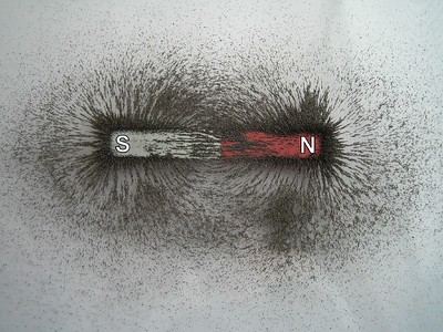
As you can see from the picture above, the bar magnet itself has two magnetic poles: north and south. The magnetic field lines go between the north and south poles. Outside of the bar magnet, the magnetic field lines go from the north pole towards the south pole. From our method of finding the direction of magnetic field lines from compasses, this means that the north pole of the compass is attracted to the south pole of the bar magnet. Much like charges, opposites attract!
Poles are not charges
Students often see this analogous behavior between electric charges and magnetic poles, and go forward and say that it is because they are equal. This is not true! Magnetic poles are not the same as electric charges. They display similar behaviors, regarding directions of forces and field lines, but they are distinct physical properties. In fact, we will see later that magnetic poles are created by the motion of electric charges.
You may also notice that the magnetic field lines never end. Instead they form loops, with each line starting at the north magnetic pole, extending outside the bar magnet to the south magnetic pole, then joining up again to itself back at the north pole. Magnetic field lines have no beginnings or ends. This is different than electric field lines, which start and stop at electric charges. This is a manifestation of a physical observation: there is no such thing as an isolated magnetic pole, they always come in north/south pairs. We refer to two opposite magnetic poles, such as a bar magnet, as a magnetic dipole. A single pole (or magnetic monopole) has never been seen, although there are theoretical reasons to expect that they may exist.
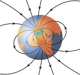
The definition of direction for the magnetic field lines has another interesting consequence. Remember that these field lines are given by which way the “north” end of a compass points. Because opposite poles of a magnet attract, this means that the north geographic pole of the Earth is where the south magnetic pole of the planet’s magnetic field is! Our compass points (roughly) north because it is attracted to a south magnetic pole! As you can see in the picture below, the magnetic field of the Earth has roughly the same magnetic dipole behavior as a bar magnet.
Problem
The magnetic field around a bar magnet is shown in the picture below. What can you say about the two poles \(A\) and \(B\)? Choose the best answer below.
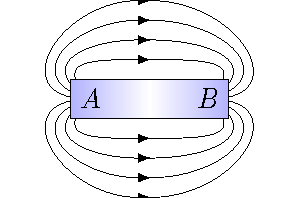
Fig. 26.3 Magnetic field of a bar magnet
\(A\) is a negative pole, \(B\) is a positive pole
\(A\) is a north pole, \(B\) is a south pole
\(A\) is a positive pole, \(B\) is a negative pole
\(A\) is a south pole, \(B\) is a north pole
Answer: \(A\) is a north pole, \(B\) is a south pole
Problem
Select the arrow that gives the correct direction of the magnetic field due to the bar magnet at the indicated point, or state that the magnetic field is zero.
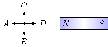
Fig. 26.4 What is the direction of the magnetic field to the left of the bar magnet?
Answer: The magnetic field at the marked point has a direction to the left (\(A\)).
Problem
Select the arrow that gives the correct direction of the magnetic field due to the bar magnet at the indicated point, or state that the magnetic field is zero.
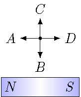
Fig. 26.5 What is the direction of the magnetic field above of the bar magnet?
Answer: The magnetic field at the marked point has a direction to the right (\(D\)).
26.3. Magnetic force
Now that we have an understanding of magnetic fields, we can use this to find the magnetic force on a charged particle. Recall that from Lesson 25, the relation between electric fields \({\vec E}\) and electrostatic forces \({\vec F}_e\) was rather simple, namely
for a test charge \(q_0\). However, the magnetic force equation is more complicated. In particular, it depends not only on the magnetic field vector and the charge itself, but also the velocity of the charge!
Quantity: Magnetic field
Symbol: \({\vec B}\)
Definition: The magnetic force \({\vec F}_m\) on a charge \(q\) moving with a velocity \({\vec v}\) is related to the magnetic field \({\vec B}\) at the charge’s location by
SI units: teslas (T)
You should probably review the vector product from Lesson 20, to make sure you know how to calculate the magnetic force from the other information given.
Problem
A proton moves perpendicular to a uniform magnetic field \({\vec B}\) with a velocity \((1.20 \times 10^7 \textrm{ m/s}) {\hat z}\) and experiences an acceleration \((2.60 \times 10^{13} \textrm{ m/s}^2) {\hat x}\). What is the magnetic field (in mT)?
Answer: \((+22.6 \textrm{ mT}) {\hat x}\)
Because of this vector product, the magnetic force \({\vec F}_m\) has some important properties. First, the magnetic force on a stationary charge is zero! It does not matter how large the charge is, if it is not moving, then there will be no \({\vec F}_m\) acting on it. Second, the direction of the magnetic force is always perpendicular to both the velocity and magnetic field vectors. Notice, however, that \({\vec v}\) and \({\vec B}\) may not be perpendicular to each other. Remember from Lesson 20 that the magnitude \(|{\vec A} \times {\vec B}| = AB \sin \theta_{AB}\), where \(A, B\) are the vector magnitudes, and \(\theta_{AB}\) is the angle between the two vectors. Then the magnitude \(F_m\) of the magnetic force is
where \(\theta\) is the angle between the velocity \({\vec v}\) and the magnetic field \({\vec B}\). It is entirely possible that the angle \(\theta = 0\) or \(\theta = 180.^\circ\), in which case the magnetic force is zero.
Problem
A proton travels with a speed of 3.00 Mm/s at an angle of 28.0\(^\circ\) relative to the direction of a 700 mT magnetic field. What is the magnitude (in N) of the magnetic force on the proton?
Answer: \(1.58 \times 10^{-13}\) N
As we did when introducing the vector product, we can use the right-hand rule (RHR) to give the relationship between the directions of the charge velocity \({\vec v}\), the magnetic field \({\vec B}\), and the magnetic force on the charge \({\vec F_m}\). This is given by the figure below. There are other right-hand rule techniques, but I like this one, since you can see how the force is perpendicular to the velocity and magnetic field. The rule is that the pointer finger is in the direction of the velocity, the middle finger in the direction of the field, and the thumb will point in the direction of the magnetic force.
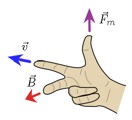
Notice this assumes that the charge is a positive charge! When you are using the RHR and have a negative charge, you can either just reverse the direction for the magnetic force, or else use your left hand. For the latter case, which finger goes with which vector is the same, just the mirror image.
As a way to represent 3D vectors on a 2D page (or screen), here is some notation. Imagine that we have an arrow, with an arrowhead on one end, and the feathers of the arrow on the other. If the arrow is coming towards you, you will see the tip of the arrow and the round arrowhead; if the arrow is going away from you, you see the four feathers at the end. We represent these with the following pictures:
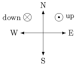
Fig. 26.7 Notation for three-dimensional vectors
Thus, a circle with a dot (or sometimes just a dot) is the tip and arrowhead coming towards you, while the cross in a circle (or just a cross) are the feathers going away from you. Here are some practice questions; remember to think three-dimensionally!
Problem
A positive charge enters a uniform magnetic field (the blue crosses in the diagram) as shown. What is the direction of the magnetic force? Choose the best answer.
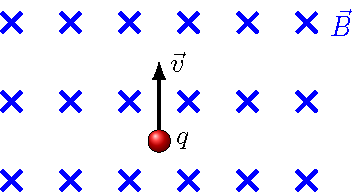
Fig. 26.8 Find the direction of the magnetic force
towards the top of the page
towards the bottom of the page
into the page
out of the page
to the left
to the right
Answer: to the left
Problem
A positive charge enters a uniform magnetic field (the blue lines in the diagram) as shown. What is the direction of the magnetic force? Choose the best answer.
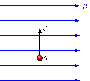
Fig. 26.9 Find the direction of the magnetic force
towards the top of the page
towards the bottom of the page
into the page
out of the page
to the left
to the right
Answer: into the page
Problem
The magnetic force on a proton points downward. If the velocity of the proton is westward, what is the direction of the magnetic field the proton moves in?
Answer: north
Problem
An electron has a magnetic force acting due west on it. If the electron is moving in a magnetic field pointing due north, what is the direction of the electron’s velocity?
Answer: down
26.4. Motion of charged particle in constant magnetic field
From the above equation for the magnetic force \({\vec F}_m\), this force is at its maximum size when the velocity of a charged particle is perpendicular to the magnetic field. Let’s explore this situation a little more; we will see that this gives interesting behavior we did not see with the electric field. In particular, since the magnetic force is perpendicular to both the magnetic field and the velocity, this means that the charge will experience an acceleration that is always perpendicular to the velocity. There will never be an acceleration along the magnetic field lines.
If you remember the ideas of circular motion from Lesson 18, you will see that this means the magnetic force acts like a centripetal force here! The magnetic force will always be pointing perpendicular to the velocity, so the charge curves around in the direction of that force, but keeping the same speed. You can see this yourself by running the program below. The cyan arrows represent a constant magnetic field, and the program simulates the motion of a charged particle in that field, with a velocity perpendicular to the field. The red arrow is the momentum of the charge.
Let’s make this more mathematical. If the magnetic force acts like a centripetal force, then we can use Newton’s second law to find out the radius of the resulting circle. Using \({\hat r}\) to be the usual radial unit vector (i.e. the unit vector at the charge, pointing away from the center of the circle), then
Recall that the minus sign here is because the centripetal force always points towards the center of the circle. However, the magnetic force will as well, so \({\vec F}_m = -F_m {\hat r}\); in this situation, the magnetic force acts like a (constant) central force. This means we can relate the magnetic force magnitude \(F_m\) to the centripetal force by
The charge \(q\) is in absolute value signs, since we are using only the magnitudes; you should think about how changing the sign would alter anything with the directions. Also, we have already assumed that the velocity is perpendicular to the field, so \(\theta = 90.0^\circ\), giving \(\sin \theta = 1\). Solving the equation for the radius of the circle, we get
Problem
For the default values in the program above, the circular motion of the charge is not centered at the origin. What speed would be necessary, so that the point \((0, 0, 0)\) is at the center of the charge’s path?
Answer: To have the path centered at the origin, the radius of the circle must be \(r = 3.00\) m (from the value of INIT_POS). Solving for the speed \(v\) in the equation above gives
so \(v = 5.00\) m/s.
Problem
What happens if you use the speed from the last problem, but change the sign of the charge \(q\)?
Answer: The charge will move in a circular path of the same radius as before, but counterclockwise instead of clockwise. Thus, the path will be centered to the left of the charge’s starting point.
Problem
Suppose you change the velocity, so that it points along the magnetic field direction. What kind of motion do you see now?
Answer: If the velocity is parallel to the magnetic field, then the magnetic force has zero magnitude. Thus, the charge will continue along a straight path.
Problem
Change the velocity, so that it has both non-zero \(y\) and \(z\) components. This means that the velocity has components both parallel and perpendicular to the magnetic field. What kind of path will the charge have?
Answer: The charge will now have a combination of motions. The magnetic force will always point in the \(x-y\) plane, so the charge will have circular motion in this plane as well. However, with the non-zero \(z\) component of the velocity, the charge will continue to move at a constant rate in this direction. The combination of the two is a helical path around the magnetic field lines.
26.4.1. The mass spectrometer
There are many cases where the circular motion of charges around the magnetic field lines occurs. One of which we depend on every day! The strong magnetic field of the Earth channels charged particles, coming from the Sun and other sources in outer space, along its field lines. This serves as a barrier for most of these charges, preventing them from hitting the Earth’s atmosphere. If they did in great numbers, this would steadily erode the atmosphere, destroying the ozone layer, and eventually stripping the Earth of its air. In comparison, it is believed that the weak magnetic field of Mars was a key factor in that planet’s loss of atmosphere; the surface pressure at the Martian surface is only about 600 pascals (compared to 101.3 kPa on the Earth!).
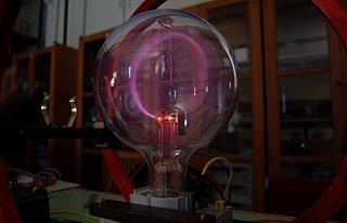
Another common use for the process described above is the mass spectrometer; you may have heard this term if you watch a lot of crime shows. A mass spectrometer takes an unknown substance, ionizes the constituents in some way, then feeds these molecules into a constant magnetic field. By determining the path of these molecules, the molecular charge-to-mass ratio \(q/m\) can be calculated. Early versions of this were used by various physicists to study “cathode rays”, those particles we now call electrons. The picture below shows such a process – the air molecules inside the tube are fluorescing because of collisions with the electron beam.
Let’s go through an estimate of how large the circular path of electrons would be in a laboratory experiment. Suppose we use a voltage \(\Delta V = 3000\) V to accelerate the electrons. Voltage \(V\) (as known as electric potential) is related to electric potential energy \(U_e\) by \(\Delta U_e = q \Delta V\), for a charge \(q\). This gives each electron a kinetic energy of \(e \Delta V = 4.81 \times 10^{-16}\) J. With the mass \(m_e = 9.11 \times 10^{-31}\) kg, then the electrons have a speed of \(3.25 \times 10^7\) m/s – about 1/10th the speed of light. Using this speed in the Earth’s magnetic field of about 50.0 \(\mu\) T, then the electrons will travel in a circular path with a radius of 3.69 m. In the picture above, a magnetic field is created which is about ten times stronger than the Earth’s field, so the path is correspondingly smaller.
Problem
Suppose you want to use a mass spectrometer to determine the ratio of U\(^{235}\) to U\(^{238}\) in a confiscated shipment. If each isotope is singly ionized and placed in a 750. mT magnetic field, with masses \(m_{235} = 3.90 \times 10^{-25}\) kg, \(m_{238} = 3.95 \times 10^{-25}\) kg, and both isotopes are moving at \(1.05 \times 10^5\) m/s, what is the distance separation (in mm) of the isotopes after half a circular orbit inside the magnetic field?
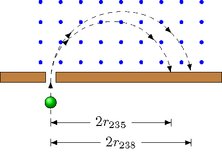
Fig. 26.11 Uranium ions in a mass spectrometer
Answer: 8.74 mm
Problem
The image below shows a particle, \(q\), as it moves through a magnetic field of \(B = 0.570\) T in a circular path with a radius of 30.0 cm. Determine whether \(q\) is a proton (\(m_p = 1.67 \times 10^{-27}\) kg) or electron (\(m_e = 9.11 \times 10^{-31}\) kg) from the image, and then use the appropriate mass in order to calculate the speed of \(q\) (in m/s) while in the magnetic field.
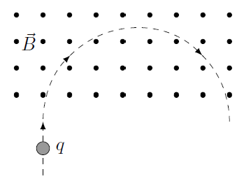
Fig. 26.12 Unknown charge moving in a magnetic field
Answer: \(1.64 \times 10^7\) m/s
Problem
An electron moves through four different regions (each represented by a different shade) from region I to region IV.
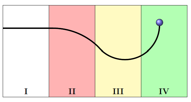
Fig. 26.13 Electron moving through four regions
Based off of the path shown, find the directions of the magnetic fields in each region. Note it may be possible that the magnetic field is zero in a particular region.
Answers: For region I, the magnetic field can either be zero, or in the left-right direction, since the magnetic force on the electron is zero. For the other three regions, the electron is undergoing uniform circular motion, so the magnetic force points towards the center of the circular motion for each region. For region II, the force is towards the bottom of the page, so the magnetic field is into the page. For regions III, the force is towards the top of the page, so the magnetic field is out of the page.
26.5. Summary
We have now introduced the last of the three types of fields we will see in this course: the magnetic field \({\vec B}\). Like the gravitational field \({\vec g}\) and the electric field \({\vec E}\), the field at a particular point is measured to have the same magnitude and direction by all observers, and is used to find the corresponding force on an object at that point. The simplest system creating these magnetic fields is the magnetic dipole, consisting of a pair of magnetic poles, one a north pole and the other a south pole. Examples of these magnetic dipoles range from a simple bar magnet to the overall structure of the Earth’s magnetic field.
In addition, we saw that a charged particle moving in a magnetic field undergoes circular motion around the field lines; if the charge’s velocity has non-zero components both parallel and perpendicular to the field, then the motion will be helical around the field lines. This has many applications, such as the mass spectrometer, as well as others in particle physics experiments.
However, we have not touched on the important question of how these magnetic fields are created. For the gravitational and electric fields, this was relatively easy. In particular, we could start with the fields due to a point mass or charge (depending on which field type we are talking about!), where the field magnitude was an inverse square law, and the direction was given by the unit vector \({\hat r}\), either in the same direction or opposite the position vector. Then, we could add together the contributions of a large number of point masses or charges to get the fields due to more complicated shapes.
As we will see in the next lesson, this basic recipe is the same, with magnetic fields created by the motion of charged particles, or currents. However, like the magnetic force equation we saw in this lesson, the field created by a “point current” involves the vector product, so it is not so simple as, say, the gravitational field of a point mass. This is dealt with using Biot-Savart law in the next lesson.
After this lesson, you should be able to:
State the direction of the magnetic field due to magnetic poles.
Interpret a drawing of magnetic field lines.
Describe the motion of a charged particle in a constant magnetic field.