.ipynb .pdf

Binder

Contents

3. Velocity and the Euler method

3.1. Overview

Links to programs in this lesson:

1. A sphere

2. The Euler method

3. Position and velocity graphs

This lesson starts with exploring the motion of objects. We will formally define quantities such as displacement and velocity to describe such motion. Later, in Lesson 05, we will talk about what happens when the velocity changes, due to an acceleration. Since a lot of what we will do in the class will depend on the ideas here, I will spend some time going through the reasoning behind them. In particular, we need to tell the computer how to take an initial position vector and a velocity vector, and update the position accordingly. So I will devote a lot of space to describing the necessary programming; this will built off of what we talked about with vectors in Lesson 02.

I will also use graphs of the motion to help quantify the motion. Graphs are an important source of information in science and engineering, and it is important that you are comfortable with them. There are some basic methods of reading graphs that you will use over and over. These will be developed in this lesson.

As a scaffolding for these ideas, we will build up a vPython simulation of a ball moving with constant velocity until it bounces against a wall, then moving in the opposite direction. We have already seen just about all of the vPython commands necessary to do this, we just need to add in some physics! So let’s get started.

Here are the objectives for this lesson:

• State the definitions of average and instantaneous velocity.

• Describe how the graphs of position vs. time and velocity vs. time for an object are related.

3.2. Creating a sphere

As mentioned above, we are going to create a moving object. To be specific, let’s create a sphere object in vPython. This is done in the Trinket app below, which has a function createSphere(). The sphere is a lot like the arrow we saw in Lesson 02, but it has some different attributes. Like an arrow, the sphere has a position pos, which is where the center of the sphere is located, and a color color. As you would probably expect, there is an attribute radius; the default value is 1, but I have made it somewhat smaller. In addition, vPython objects have the helpful property that you can add your own custom attributes to any object. I have added the attribute velocity to the sphere, to give it a velocity pointing to the right.

Back to program list

However, if you run the program above, the sphere doesn’t move! Why is that? That’s because just creating an attribute velocity is not enough to get the ball moving. We have to add in the code that uses the velocity vector in changing the position of the sphere. This process is known as updating the position.

Now we start studying the idea of “velocity”. You probably have an intuition of what this means, but this is one topic where the common ideas of what “velocity” and “speed” mean are not good enough for use in physics. Thus, it is really important to be aware of what the definitions of these quantities are, and how they differ from what we use in everyday speech. To set this up, first we need some other definitions first.

3.3. Creating motion

We are so used to movies, TV shows, and videos that we don’t really think about the fact that they are showing us an artificial view of the action. Specifically, the cameras used to make these productions are not filming everything that happens, but instead are taking pictures of what is in front of them at a certain frame rate. For example, a movie camera may capture a frame 24 times a second. This is a rapid enough rate so that when these pictures are shown to humans, they look like continuous motion. You only ever notice the difference if the frame rate is slowed down.

Suppose you are filming the next great American movie, and it features a scene with a ball moving at a constant velocity. Again, your camera is only going to record the ball’s position at certain times, which I call \(t_n\) here. The starting position is at time \(t_0\), and \(t_n\) is the time after \(n\) additional frames have been recorded. If the time between frames is called \(\Delta t\), then \(t_n = n \Delta t\). This quantity \(\Delta t\) is called the time interval. At each \(t_n\), the ball is at a position vector \({\vec r}_n\), as seen by your camera at the origin \(O\). This set-up might look like the picture below.

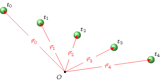
Fig. 3.1 Film frames of a ball moving at constant velocity

The frames record the position of the ball only at these moments \(t_n\). If you use a frame rate of 24 frames per second, then after one second, you have taken 24 frames. This means the time interval \(\Delta t\) is 1/24 seconds, or about 0.0417 seconds per frame. This gives pretty smooth motion when projected onto a screen.

The symbol “\(\Delta\)”

Often in physics, we will care about the difference of a particular quantity. This is given by the symbol \(\Delta\). So, for example, when I said the change in time is \(\Delta t\), you can think of this as the time elapsed between one frame and the next; this would be the difference in the initial time \(t_i\) and final time \(t_f\), so

\[ \Delta t = t_f - t_i \]

Anytime you see \(\Delta\), you should automatically think “final minus initial”. This could be used for differences in vertical position \(r_y\),

\[ \Delta r_y = r_{f, y} - r_{i, y} \]

changes in energy \(E\) of a falling rock,

\[ \Delta E = E_f - E_i \]

or voltage differences \(V\) for an electron passing through a battery,

\[ \Delta V = V_f - V_i \]

Now, what if you can’t get anyone to fund your movie, and you decide to become a video game developer? On the surface, your goal is the same: create pictures of the motion rapidly enough so that the motion looks realistic. However, there is a subtle difference in what you are trying to do here. With your movie, you are filming something happening “in real life”, so you are taking frames of an already existing object. For your game, however, you are simulating the motion of an object that does not really exist! In other words, you have to work out what kind of motion is realistic, and show that motion to the game player at a frame rate so that everything looks like reality.

This is what we are trying to accomplish in vPython with our simulations as well – create realistic motion using physics principles. Much like the film maker, we have to show this motion as a series of pictures at a certain frame rate. But, like the video game developer, we do this by computing the positions of objects, rather than simply recording them. So how do we do this?

3.4. Displacement

To set up how we will create realistic motion using vPython, we need to get a couple of important definitions under our belt. The first of the quantities we will define is displacement; we saw this in Lesson 02, but we will now define it. The displacement is a vector quantity giving the straight-line distance between the starting (\({\vec r}_i\)) and ending (\({\vec r}_f\)) points, i.e. “as the crow files”. Thus, it is an easy quantity to work with – if an object moves through some path, to find the displacement, it does not matter what the path is, just the beginning and end of it. Obviously, objects can move through some very convoluted paths due to forces acting on them, so why is the particular trajectory not important? I can give you two answers for this, depending on the situation. For some, such as a basketball thrown out onto the court, the effect of gravity will result in only one possible path from your hands to where the ball lands; if I know the displacement of the ball, I can calculate everything else about the motion (such as time of flight, initial velocity). For other situations, this may not be clear. However, I can think of the complicated path as a big number of small displacements put together, one after the other. This is where using a computer is great – I can tell the computer what the rules are for each displacement, and it will find the trajectory of the object. An example of this is if I threw a feather out on the basketball court instead. If I tell the computer the rules for both gravity and air resistance, it can find the overall displacement as the sum of a bunch of individual pieces.

Whenever we define a new physical quantity, I will provide a list giving some important information about it; here is the list for displacement.

• Quantity: displacement

• Symbol: \(\Delta {\vec r}\)

• Definition:

\[ \Delta {\vec r} = {\vec r}_f - {\vec r}_i \]

• SI units: meters (m)

First, note that the position is given by the symbol \({\vec r}\). Unfortunately, physicists don’t reall have a standard symbol for distance, so you may see \(r\), \(d\), \(x\), \(y\), \(s\), … I will fix my notation so that \({\vec r}\) always represents a position vector.

However, it will be important here to know that vectors have direction. Hopefully, you can already see this when you plug numbers into the equation above. If \(r_{i, y} = 3\) and \(r_{f, y} = 5\), then \(\Delta r_y = 2\), while if the initial and final numbers are reversed, then \(\Delta r_y = -2\). When the displacement \(\Delta r_y\) is positive, the object has moved in the positive direction, while the negative displacement means the motion was in the negative direction. So already, you can see how direction will be taken into account in physics quantities.

In the picture below, I have used the moving ball example we saw from your short film career, and added on the displacement vectors between each frame of the movie. The index \(n\) refers to the frame number in the film, starting at frame zero.

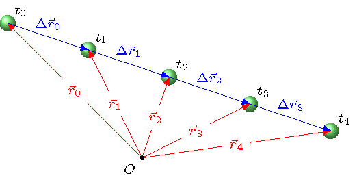
Fig. 3.2 Moving ball with displacement vectors

Notice that at each frame, there is a vector sum going on: the initial position vector \({\vec r}_n\) at one frame, plus a (constant) displacement vector \(\Delta {\vec r}_n\), gives the final position \({\vec r}_{n + 1}\) at the next frame. Written as an equation

\[ {\vec r}_{n + 1} = {\vec r}_n + \Delta {\vec r}_n \]

Again, the \(n\) in this equation is an index for which time step we are at; the index \(n\) starts at 0, and increases by one after a time interval \(\Delta t\) passes, so this is the same as

\[ {\vec r}_1 = {\vec r}_0 + \Delta {\vec r}_0 \]

then

\[ {\vec r}_2 = {\vec r}_1 + \Delta {\vec r}_1 \]

and so on. We will use this equation again, but change it slightly to include the velocity of the object; this will allow us to get our vPython sphere moving.

Problem

Rank the magnitudes of the displacements for the four paths shown in the figure below, from greatest to least. For example, a possible ranking is \(1 > 2 = 3 > 4\).

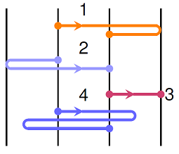
Fig. 3.3 Four paths, with equally spaced lines

Answer: All four motions involve moving one unit to the right, even though some requirement a greater total distance traveled than others. Thus, both the size and direction of the displacements are the same, so the ranking is \(1 = 2 = 3 = 4\).

Let’s now start looking at this in terms of graphs. In the figure below, the motion of the ball is placed on top of a grid of points. At each time \(t_n\), the coordinates \((r_x, r_y)\) of the ball can be read off the graph. For example, at \(t = t_0\), the ball is at \((-5, 5)\) m. Notice that you have to use the given labels on the axes to figure out these values; each grid square is one meter, both in the \(x\) and the \(y\) directions.

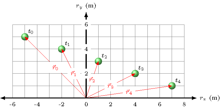
Fig. 3.4 Moving ball on a position grid

Problem

Find the coordinates for the ball at the remaining times \(t_n\), and fill in these values into the table below.

Time	\(r_x\) (m)	\(r_y\) (m)
\(t_0\)	-5	+5
\(t_1\)
\(t_2\)
\(t_3\)
\(t_4\)

Answer: The completed table is given below.

Time	\(r_x\) (m)	\(r_y\) (m)
\(t_0\)	-5	+5
\(t_1\)	-2	+4
\(t_2\)	+1	+3
\(t_3\)	+4	+2
\(t_4\)	+7	+1

This will be your first graph skill: reading the graph. Here, to get the ball’s coordinates, you simply read the values off the graph. Since this is a position graph, the numbers you read off are simply the \(x\) and \(y\) positions of the ball at various times \(t_n\). However, we will usually not see motion given in this form. A more typical graph would be of position vs. time. The \(x\) position vs. time graph for the ball is given below.

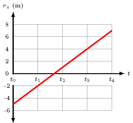
Fig. 3.5 \(x\) position vs. time graph for the ball

Notice that I don’t include the ball itself anymore; the graph below will be the usual format you see them in. However, reading the graph is the same as before, but now, you can see the \(x\) position \(r_x\) of the ball at a given time, or vice versa. You should check to make sure you can verify your answers for the table from the graph.

Problem

Which of the following graphs correctly represents the graph of the \(r_y\) position of the ball as a function of time?

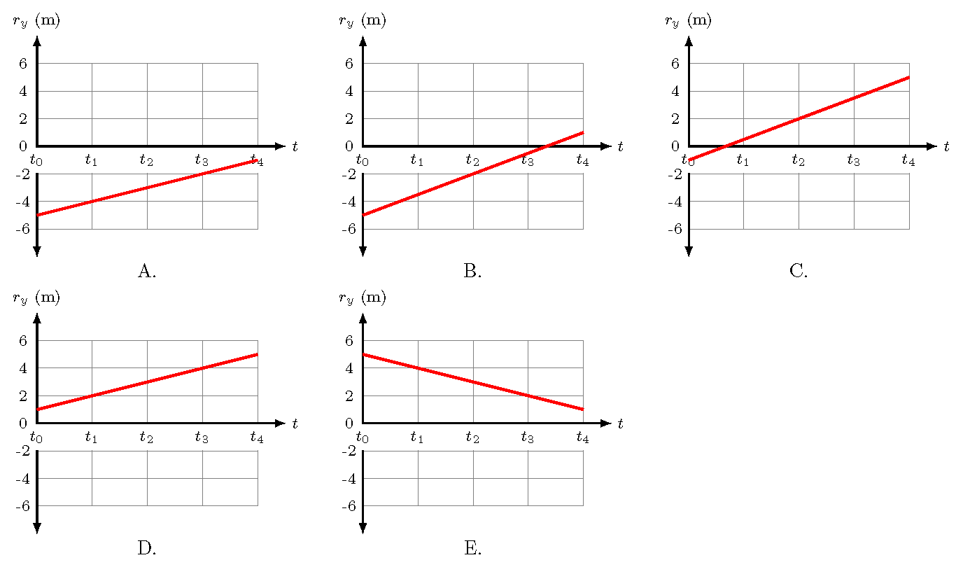
Fig. 3.6 \(y\) position vs. time graph for the ball

Answer: Between time \(t_0\) and time \(t_4\), the ball moves from a position \(r_y = +5\) m to \(r_y = +1\) m. The only graph that matches these values is graph \(E\).

3.5. Velocity

Let’s now build on our definition of displacement and come back to the moving ball. Remember that the displacement vectors for the ball are all the same. Other than the fact we have shifted the location of their tails, they all have the same size and direction. Why is this? Well, it stems from the fact that the velocity of the ball is constant: the ball is moving with the same displacement \(\Delta {\vec r}\) every time interval \(\Delta t\). This leads to the definition of average velocity as a vector given by displacement over time elapsed.

• Quantity: average velocity

• Symbol: \({\vec v}_{avg}\)

• Definition:

\[ {\vec v}_{avg} = \frac{\Delta {\vec r}}{\Delta t} = \frac{{\vec r}_f - {\vec r}_i}{\Delta t} \]

• SI units: meters per second (m/s)

Notice that average velocity is a vector, since the displacement was! As I mentioned in Lesson 02, \({\vec v}_{avg}\) is found by the scalar multiplication of \((1/\Delta t)\) and \({\vec r}\).

Instead of showing the difference in positions with the constant displacement vector \(\Delta {\vec r}\), we can write it in terms of the velocity \({\vec v}\) of the ball; since the ball’s velocity is constant, I have dropped the “avg” subscript. From the definition of velocity, \(\Delta {\vec r} = {\vec v} \Delta t\), so the position of the ball at each frame can be found with

\[ {\vec r}_{n + 1} = {\vec r}_n + {\vec v} \Delta t \]

This is shown in the figure below.

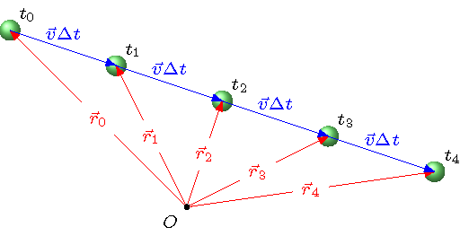
Fig. 3.7 Moving ball in terms of velocity vectors

It is important to note that there are many average velocities to talk about in this picture. The figure itself gives the displacements \({\vec v} \Delta t\) between successive positions, but there is also the average velocity over the entire motion shown. In this case, the two would be exactly the same – the ball maintains a constant velocity, so the only difference in displacement is from the longer time measured. Here, the total displacement is four times a given individual displacement, but that is because this is over four times the time interval of those individual motions.

However, whenever the velocity is changing, this is no longer true; this will be a concern, starting with Lesson 05, when we discuss acceleration. It is good to start thinking about it now, so you have a good conceptual grasp of what the average velocity equation means. The average velocity can be different, depending on the time interval it is taken over. An example of this is shown below. Because of the curved path the ball travels on, the displacements \({\vec r}_n\), and therefore the velocities \({\vec v}_n\), point in different directions at different times.

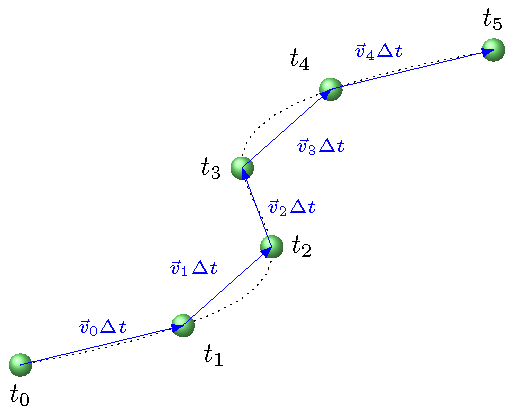
Fig. 3.8 Moving ball with changing velocity

If we imagine the frames of a movie again, increasing the frame rate will give a more accurate velocity vector at a particular time, rather than for the entire path. This process would mean taking the time interval \(\Delta t\) as small as possible; thinking like a mathematician for a moment, this means

\[ {\vec v} = \lim_{\Delta t \to 0} \frac{\Delta {\vec r}}{\Delta t} \]

The vector obtained here is known as the instantaneous velocity \({\vec v}\) – notice that I have dropped the subscript “avg” again! I could get away with it earlier, since the average velocity was the same as the instantaneous velocity, for the ball moving with constant velocity. Whenever I say “velocity”, I really mean “instantaneous velocity”.

Speed vs. velocity

You might notice that I have scrupulously avoiding using the word “speed”. For the rest of the year, I will use speed as an abbreviation for the magnitude (or size) of the instantaneous velocity; this means the information about direction has been dropped. When I say a car has a speed of 65 mph, I am not worried about which direction this motion is in. This will be a scalar quantity, so no vector sign: the speed is denoted as \(v\). This is different than the velocity \({\vec v}\), so make sure you write down the right symbol!

Problem

The picture below shows the positions of a ball moving in a circle at various times \(t_n\). Use the labeled directions to answer the following questions.

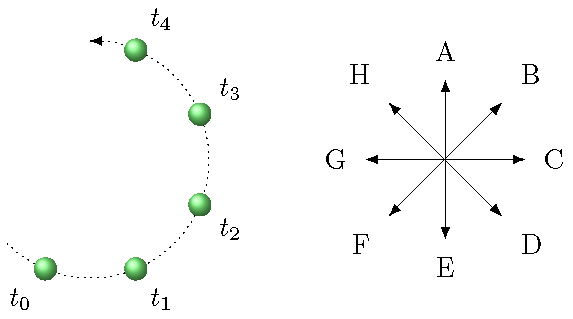
Fig. 3.9 Ball moving in circular motion, with positions marked at times \(t_n\)

1. What is the direction of the average velocity between times \(t_0\) and \(t_1\)?

2. What is the direction of the average velocity between times \(t_2\) and \(t_3\)?

3. What is the direction of the average velocity between times \(t_0\) and \(t_3\)?

Answers: All of the average velocity vectors have directions which are found by starting at the position of the ball at the initial time, and moving in the direction of the final position. From the direction of the motion given, we have that \(t_0 < t_1 < \cdots < t_4\). Thus, the average velocity between \(t_0\) and \(t_1\) is in the direction \(C\); the average velocity between \(t_2\) and \(t_3\) is in direction \(A\); the average velocity between \(t_0\) and \(t_3\) is in direction \(B\).

3.6. The Euler method

We will now implement these ideas into the vPython simulation we had before for the ball. The basic program is given below, and I will explain it in a moment. However, note that it is incomplete – you will have to add in the crucial commands necessary to get the ball to move!

Back to program list

Variable types

If you are interested in learning more about computer programming, then the point I make here about variable names is an important one. Variables that are defined inside Python procedures and functions are called local variables, and are only defined within that group of code; the computer does not know what they are outside of the procedure or function they are originally set in. On the other hand, variables in the main program are called global variables, and can be used anywhere inside the program, including the procedures and functions. This is why giving local and global variables the same name can be confusing – you may want to use a variable in the main program that is only defined inside a function! There are ways around this, but they may make the issue worse if you are not careful.

In the program above, I have copied the function createSphere() from the first program in this lesson, and changed it slightly. Now, it takes arguments start_pos and start_vel, the initial position and velocity vectors, respectively. This allows you to play around with these values if you wish, and see how the motion changes. For this particular program, though, I have defined the variables INIT_POS and INIT_VEL at the top of the program. Note that the variable names here do not have to be the same as those inside the function; in fact, it is a good idea to make them different, since confusing them may cause problems. You will notice I also did this when using new_sphere inside the function, but ball when calling it in the main program. Also, I like to put my variable definitions all together towards the top of the program, so it is easy to find and change them, if necessary. Along these lines, when I call the function createSphere(), I assign it to the variable ball, so that the sphere object created in the function, I have a name I can use to change its position later in the program.

Now, let’s get into how to change the ball position. The process of changing a variable, based on some mathematical relation, is known as updating. Here, we will use the equation we had earlier, namely

\[ {\vec r}_{n + 1} = {\vec r}_n + {\vec v} \Delta t \]

Remember that the index \(n\) here refers to the number of time steps \(\Delta t\) that have passed. In other words, the total time \(t = n \Delta t\). Using the film analogy again, \(n\) is the number of movie frames that we have gone through, while \(\Delta t\) is the time between showing each frame on the screen. We have to put this into vPython commands in the program above.

Let’s start with updating the ball position. First, remember from Lesson 01 what it means when we use the command x = x + 1 in Python: the computer sees what the current value is for the variable x, adds one to that value, then puts the new value back into the variable x. This command updates the old value x to get a new value x equal to one greater than the one. We are doing something similar with the equation above: we start with the old value \({\vec r}_n\) of the ball’s position vector, we add \({\vec v} \Delta t\) to it, then make that sum the new value \({\vec r}_{n + 1}\) of the ball position. This guides us in how to update the ball position! With the time step DT in the program, we want to use the command

ball.pos = ball.pos + ball.velocity * DT

Remember that, if you wish, you can abbreviate the command a bit using the Python operator += to write

ball.pos += ball.velocity * DT

Type in either of these commands into the program above, but don’t run it yet!

This programming command comes straight from the physics definition of velocity. This method of updating the ball position is known as the Euler method, where we take an equation of the form

\[ B = \frac{\Delta A}{\Delta t} = \frac{A_{new} - A_{old}}{\Delta t} \]

and find the new values of \(A\) by “stepping” this equation in the form

\[ A_{new} = A_{old} + B \Delta t \]

Later on in your academic career, you may see equations like this, but as derivatives of functions in calculus class. There, you can try to find the actual function for all times that satisfies the equation. However, we are doing it numerically, using a computer, so we need a method to compute the values at different times. This is why we need a technique like the Euler method.

So why don’t I want you to run the program yet? Well, notice that the while loop will run until the desired time period MAX_TIME is complete. But where does the time elapsed t get changed in the program? So far, nowhere! Thus, we need to update the time as well. This is why I reminded you above about the relationship between total time \(t\) and the time step \(\Delta t\). We need to move on to the next time interval by using

t = t + DT

or

t += DT

This will change the “clock” of the simulation from \(t_n = n \Delta t\) to \(t_{n + 1} = t_n + \Delta t =(n + 1) \Delta t\). Add in this code to the program.

Tempus fugit

One common error I often see is that students forget to include this statement that changes the time variable t. Then they run the program, and it looks like the computer has frozen! Instead, the computer is running exactly what you told it to, to change the position ball.pos but not the time. So the while loop never stops, since the condition t < MAX_TIME is always satisfied. Don’t forget this part!

Run the code and see what happens now. Looks like nothing, right? And why is the ball on the right-hand side of the screen? Because computers are very fast, the ball moved so fast that you saw only a flash! To slow down the animation, insert the statement rate(100) inside the loop, where it says to set the computer frame rate, indented as usual. This specifies that the while loop will not be executed more than 100 times per second, even if your computer is capable of many more than 100 loops per second. The way it works is that each time around the loop VPython checks to see whether 1/100th of a second has elapsed since the previous iteration. If not, VPython waits until that much time has gone by. This ensures that there are no more than 100 iterations performed in one second. Note that this frame rate is different than the one we set ourselves with the value DT; rate() sets the number of times the computer shows the results, while DT is related to the “internal clock” of the simulation itself, i.e. where things stand in terms of the motion there.

Now run your code. You should see the ball move to the right, with a constant velocity in the \(+x\) direction.

Problem

Experiment with changing the arguments for createSphere(), and see how the motion changes. Specifically, change the values of either variable INIT_POS or INIT_VEL, and rerun the program.

Problem

Change the code so that the ball moves for a longer period of time. If you calculate the final position of the ball, does it match the results of the computer? How would you tell?

Answer: After the while loop (i.e. at the end of the programming, without indentation), add a print(ball.pos) command. Compare the value printed out to the one you calculate using the definition of average velocity. They should be very close to each other; the differences come from numerical error in the computer.

3.7. Slope and area under the curve

What this updating method is doing can also be seen in terms of graphs. On the left-hand side of the picture below, you will see the velocity \(v_x\) in the \(x\) direction versus time \(t\) graph for our ball. Because this object has a constant speed, the graph is of a straight, horizontal line. However, the graph also includes an interpretation for our updating equation above. Notice that we start with a position \(r_{n, x}\) and add a change \(\Delta r_{n, x}\) to it, so we know what the position is at the next time step. If you look at the Euler method equation, hopefully you can see that this change is simply given by

\[ \Delta r_{n, x} = v_{n, x} \Delta t \]

If I look at the velocity graph, this change in position is just the area of each of the marked rectangles! The rectangles have a width \(\Delta t\) in the horizontal direction, and a height of \(v_{n, x}\) in the vertical direction. It terms out this is a general rule in mathematics:

From velocity to displacement

The area under the curve for the graph of a velocity component vs. time is the component of the displacement \(\Delta r\) for the object. For example, the area of a \(v_x\) vs. \(t\) graph is the component \(\Delta r_x\).

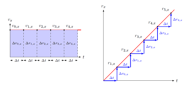
Fig. 3.10 Updating the position of the object for a constant velocity \(v_x\)

Note that this is a general rule, not just for when the velocity is constant. This is our second graph skill, area under the curve. First, note that “under the curve” means between the curve on the graph, and the horizontal axis. Thus, for a \(v_x\) vs. time graph, this is the area between the \(v_x\) curve and the \(t\) axis. Second, you can always figure out what the area is by using the units. Going back to the \(v_x\) vs. \(t\) graph, with \(v_x\) in meters per second and \(t\) in seconds, then the area is (m/s)(s) = meters. This is why we said above that the area under the curve for a \(v_x\) vs. \(t\) graph is a displacement, since it has units of position. Finally, since this area is over a change in time, the area itself must represent a change as well; the area under the curve is a displacement \(\Delta r_x\), not a position \(r_x\) at a particular time.

We now have two physics quantities defined – displacement and average velocity – and a method of finding the displacement from a velocity vs. time graph. Use these definitions to answer the following questions.

Problem

Use the \(x\) velocity vs. time graph below to answer the following questions:

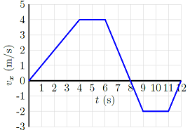
Fig. 3.11 The \(x\) velocity vs. time graph for an object

1. What is the displacement (in m) of the object from \(t = 6.00\) s to \(t = 8.00\) s?

2. What is the displacement (in m) from \(t = 8.00\) s to \(t = 12.0\) s?

3. What is the average velocity (in m/s) of the object from \(t = 0.00\) s to \(t = 8.00\) s?

Answers: \(+4.00\) m; \(-6.00\) m; 2.50 m/s

Turning to the graph on the right-hand side of the figure above the last problem, we have the position \(r_x\) versus time \(t\) graph of the ball. Here again, the time steps \(\Delta t\) and the changes in \(x\) position \(\Delta r_{n, x}\) are marked on the graph. If I move forward in time one time step, I move to the right on the graph. Since the \(x\) velocity is positive, when I move forward one time step, I move in the positive direction vertically along the graph to find my new position \(r_x\). From this, hopefully you can also see a second mathematical fact from this position vs. time graph:

From position to velocity

The slope of a position component vs. time graph is the appropriate velocity component for an object. For example, the slope of a \(r_x\) vs. \(t\) graph is the velocity component \(v_x\).

This is our third graph skill, the slope of a graph. Remember that the slope is defined as “rise over run”, i.e. the change in the quantity along the quantity displayed vertically on the graph, divided by the change in the quantity shown horizontally. For a \(r_x\) vs. \(t\) graph, this would be the \(x\) component of the average velocity, since

\[ \frac{\Delta r_x}{\Delta t} = v_{avg, x} \]

Since the slope is found using two points on the graph – in order to find the change between those two points – we need to spell out how to do this, especially with the difference between average and instantaneous quantities, like velocity. The average velocity is written exactly in the form of a slope for a position component vs. time graph, so \(v_{avg, x}\) is just the slope of the line between the initial and final \(x\) positions of an object. A straight line that intersects a given curve at two points is known as a secant line; an example is shown in the figure below. Here the secant line meets the \(r_x\) curve at the initial \(r_{i, x}\) and final \(r_{f, x}\) positions for a given time interval.

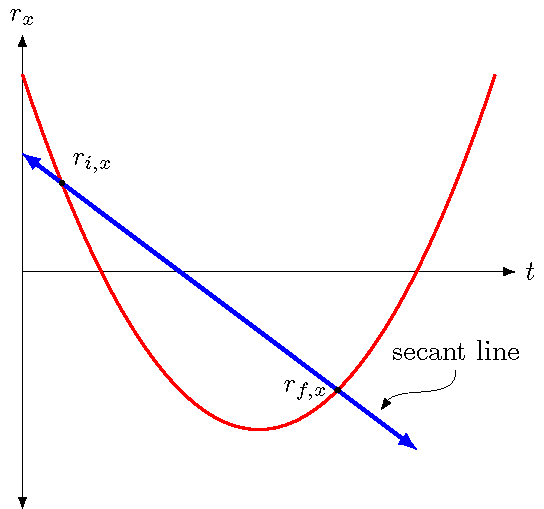
Fig. 3.12 Secant line to find average velocity

So how do we find the instantaneous velocity at a particular time? Remember this is suppose to be the velocity “at” this time, but you can’t find a slope with only one point! This is why we have the limiting process in our definition of \({\vec v}\) above. This is shown in the figure below, where we find the slope at the point \(r_x\) by starting with a secant line through \(r_{1, x}\). Then we “slide” this point closer to \(r_x\), through \(r_{2, x}\) and \(r_{3, x}\); this is what the limiting process means.

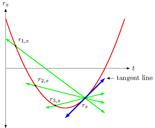
Fig. 3.13 Limiting process to find the tangent line at a point, for the instantaneous velocity at that point

The result is a tangent line: the line found through this limiting process to approximate the slope of the curve at a given point. Notice that the tangent line may have the same slope as the curve, if the curve is just a straight line! However, if the curve is really curve, the tangent line will touch the curve at only the point we are interested in.

Problem

The \(x\) position vs. time graph of an object is given below. To answer the following questions, read the graph position for the signs of the position, and estimate the slope for the velocities.

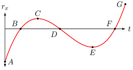
Fig. 3.14 The \(x\) position vs. time graph for an object

1. For each of the marked points, is the \(x\) position \(r_x\) positive, negative, or zero?

2. For each of the marked points, is the \(x\) velocity \(v_x\) positive, negative, or zero?

Answers: The \(x\) position component \(r_x\) is positive for points \(C\) and \(G\), negative for points \(A\), \(E\), and zero for points \(B\), \(D\), and \(F\). The \(x\) velocity component \(v_x\) is positive for \(A, B, F\), and \(G\), negative for \(D\), and zero for \(C, E\).

Problem

Use the \(r_x\) vs. \(t\) graph below to answer the following questions:

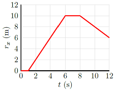
Fig. 3.15 The \(x\) position vs. time graph for an object

1. What is the displacement \(\Delta r_x\) (in m) of the object from \(t = 6.00\) s to \(t = 8.00\) s?

2. What is the displacement of the object (in m) from \(t = 1.00\) s to \(t = 6.00\) s?

3. What is the instantaneous velocity (in m/s) of the object at \(t = 10.0\) s?

4. What is the displacement (in m) from \(t = 4.00\) s to \(t = 10.0\) s?

5. What is the average velocity (in m/s) of the object over this last time interval?

Answers: 0.00 m; +10.0 m; -1.00 m/s; 2.00 m; 0.333 m/s

3.8. Graphing the motion

Now that we have a moving ball, let’s see if we can create graphs of position vs. time, and velocity vs. time, in vPython to match those used earlier when we were discussing the Euler method for updating position. Below is what your code should look like from the previous Trinket app, after you got the sphere moving. There are also spaces in the program to add in curves on a graph, using the vPython modules graph and gcurve. The instructions below the app will guide you through that process; remember you can get to the code by clicking on the pencil icon in the menu bar for the Trinket app.

Back to program list

The first graph we will create will be the \(x\) velocity \(v_x\) vs. time. To do this, we need to (1) tell the program to create a graph, and (2) plot the points for the vertical position at each time. To create the graph, add the following statements in the “Create graph and curves” section:

xGraph = graph()
xVelCurve = gcurve(graph = xGraph, color = color.blue)

The first line tells the computer to create a graph xVelGraph with the default settings; later we will change these settings to better suit our graphs. The second line tells the computer to use the graph xGraph to create a cyan curve called xVelCurve. The points on this curve will be given by the next line we will add. These commands are separate because you can, for example, add multiple curves to the same graph.

Inside of the while loop, in the section “Update curve”, add the line (remember it must be indented!)

xVelCurve.plot(t, ball.velocity.x)

to plot each new point as the computer calculates it. This line first tells the computer to update the curve xVelCurve on the graph xGraph by changing its xVelCurve.plot attribute. This update adds a point on the graph curve with horizontal coordinate t, and vertical coordinate ball.velocity.x (the \(x\) component of the velocity) – both inside the ordered pair (t, ball.velocity.x).

Run the code and see what happens. You should still see the animation of the ball moving to the right, but in addition, there should be a graph at the bottom of the page. Is the final shape of the graph what you expected?

Because we have not told the computer how big the graph will eventually be, it will continually update the size, so the numbers on the side and bottom of the graph will change until the animation is done. We can do this by changing the attributes inside the definition of xGraph. Change this definition so it now reads

xGraph = graph(xmin = 0, xmax = 3, ymin = -4, ymax = 4, xtitle = 'Time (s)', \
               ytitle = 'v_x (m/s)')

Run the program again, and you will see the grid now stays motionless as the blue line showing \(v_x\) gets longer from left to right.

Now let’s do the same thing for the \(x\) position coordinate \(r_x\). We will reuse the graph xGraph, so that both lines will appear on the same graph. Go back to the code above, and complete the following steps:

1. Create a curve xPosCurve in the “Create graph and curves” section; make the line red.

2. In the “Update curves” section, update the xPosCurve to graph the \(x\) coordinate ball.pos.x of the ball.

3. Finally, we don’t want the graph to have the vertical axis labeled with \(v_x\), since we now have two curves on the same graph. Remove the definition for ytitle inside xGraph. Instead, inside the definition for xVelCurve, add an attribute label = 'v_x (m/s)'. For xPosCurve, add label = 'r_x (m)'.

Once you have done all of these steps, run the program again, and see if the two curves look correct. Your graph should look like the one shown below. The blue velocity curve is a straight, flat line at \(v_x = 2\) reflecting the constant \(x\) velocity component of the ball. On the other hand, the ball starts with an initial \(x\) position of \(r_x = -3\), and then moves to a final \(x\) position of \(r_x = +3\) when \(t = 3\). Because the \(x\) velocity is constant and greater than zero, the red position line has a constant, positive slope.

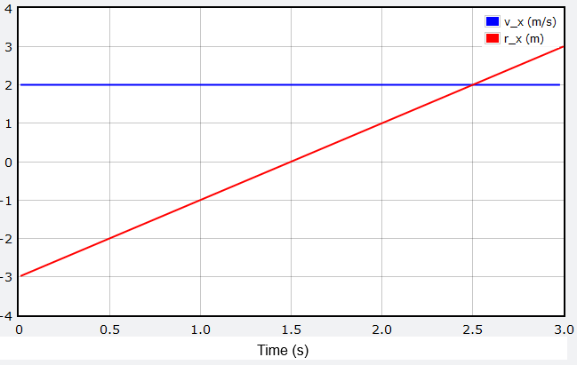
Fig. 3.16 \(x\) position and velocity of the ball as a function of time

Problem

What would the graphs look like if \(v_x\) was negative? If \(v_x\) was zero?

3.9. Summary

This lesson has two major pieces. The first part covered displacement, as well as average and instantaneous velocity. These concepts were defined, and various relationships between them laid out. This includes how to get displacement from a velocity vs. time graph, and velocity from a position vs. time graph.

The second part covered the vPython package, using it to create a sphere object. A good reference for this package is at vPython.org. We talked about the attributes of objects like this, and how they can be defined. Then, from the definition of average velocity, the Euler method enabled us to animate the sphere, so it moved at a constant velocity. This included the use of a while loop for updating the position of the sphere. Finally, the position and velocity components of the sphere were graphed using the graph and gcurve modules in vPython.

After this lesson, you should be able to:

• Define average velocity and instantaneous velocity.

• Describe the Euler method.

• Create a sphere in vPython, and update its position.

• Create a graph in vPython.

2. Vectors and vPython 4. Units and scientific notation