.ipynb .pdf

Binder

Contents

6. Kinematic equations

6.1. Overview

We now have the definitions of average velocity and acceleration from previous lessons. Taking the limit \(\Delta t \to 0\) gives the instantaneous velocity and acceleration; in graph terms, this would be the slope at a particular time on a position vs. time or velocity vs. time graph, respectively. Up until now, we have focused more on understanding what velocity and acceleration mean, and how to code them into a computer simulation.

Our next step is to view these quantities from a more mathematical side. Building from the basic definitions, we will see that there are equations that relate them to each other. Specifically, we will assume constant acceleration, and see where that takes us. In particular, we will go through the important examplem of free fall, where an object is moving along a vertical line due to the gravitational field. You have seen how to simulate this in vPython in Lesson 05; in this lesson, we will focus more on the calculational side. Then, if we wish, we can use the kinematic equations to verify the results we obtain in our simulations.

Here are the objectives for this lesson:

• State the kinematic equations, and explain when they are valid.

• Calculate an unknown vector quantity (position, velocity or acceleration) using the vector kinematic equations.

• Calculate an unknown vector component using the appropriate scalar kinematic equation.

6.2. Vector kinematic equations

For now, we assume the acceleration of the object is constant. This will allow us to derive a set of equations to use to solve for an unknown quantity. Later we will explore non-constant accelerations, using vPython programming and numerically calculating velocity and position. I emphasize the latter point because, as a general rule, it is important to know when a particular equation “breaks”. In other words, just like an engineer must find the safety margins for a particular structure or piece of equipment, you should know when an equation is valid or not. So, our key assumption here, to repeat, is that

\[ {\vec a} = {\vec a}_{avg} = \textrm{constant} \]

We can build up all the kinematic equations from this one assumption, and the definitions of average velocity and acceleration. Starting from the definition of acceleration, we get our first equation; we will also use the symbol \(t\) to represent \(\Delta t\).

\[ {\vec a} = \frac{\Delta {\vec v}}{\Delta t} = \frac{{\vec v}_f - {\vec v}_i}{t} \]

This gives

\[ {\vec v}_f = {\vec v}_i + {\vec a} t \]

Note this vector equation is the same as an equation for each of the vector components:

\[ v_{f, x} = v_{i, x} + a_x t \qquad v_{f, y} = v_{i, y} + a_y t \qquad v_{f, z} = v_{i, z} + a_z t \]

It is simpler to write the vector equation (three equations for the price of one!), but realize that it means the equation must be satisfied in each of the coordinate directions.

Another point is that we have been using this kinematic equation already when updating the velocity of an object in vPython. In Lesson 04, when we found the final velocity ball.velocity of an object ball at the end of a time step DT, with acceleration ball.accel, then

    ball.velocity += ball.accel * DT

So hopefully you see the relationship between physics and computing when we construct simulations. However, we can go further in the simulations, even when the acceleration is not constant. In a case like that, the new velocity would be just an estimate, since the kinematic equation is no longer exactly accurate, and there would be some error in our computations. Reducing that error as much as possible is a key pursuit in computational physics.

For the next problem, one of the givens is not provided explicitly in the statement, but you need it to do the calculation. Think about what is happening when you reach the time you are solving for. Often, there are such implicit numbers necessary in solving the problem. We will see this more as we go through free fall and, later, projectile motion in Lesson 07.

Problem

A rabbit runs across a meadow. A scientist watching the rabbit through a surveillance camera sees the following motion:

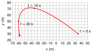
Fig. 6.1 The motion of a rabbit

The velocity of the rabbit at \(t = 0\) is \((-9.10 \ \text{m/s}) {\hat x} + (7.20 \ \text{m/s}) {\hat y}\), and the rabbit’s acceleration is \((43.6 \ \text{cm/s}^2) {\hat x} + (-62.0 \ \text{cm/s}^2) {\hat y}\). At what time (in s) does the rabbit momentarily stop in the \(y\) direction? Note that the rabbit is still moving in the \(x\) direction!

Answer: 11.6 s

Problem

Write a vPython function rabbitStop() that finds the time when the rabbit’s motion switches directions in the \(y\) direction. Assume, as in the problem above, that the rabbit has a constant acceleration, and that the initial \(y\) velocity component of the rabbit is positive. The arguments of the function are two vPython vectors: init_vel, the rabbit’s initial velocity, and accel, the acceleration. The function should output the time when \(v_y\) goes from positive to negative. You should check your results using the numbers from the previous problem.

Answer: Here is one possible program to simulate the rabbit.

def rabbitStop(init_vel, accel):

    # Create spherical rabbit
    
    rabbit = sphere(pos = vector(0, 0, 0), velocity = init_vel, \
                    accel = accel)

    # Time definitions (in seconds)

    t = 0
    DT = 0.01

    # Evolution loop

    while rabbit.velocity.y > 0:
    
        # Update rabbit position, velocity
        
        rabbit.velocity += rabbit.accel * DT
        rabbit.pos += rabbit.velocity * DT
        
        # Update time
        
        t += DT
        
    # Return time to switch v_y sign
        
    return t

You can check your results against the problem above by running the commands

result = rabbitStop(vector(-9.10, 7.20, 0), vector(0.436, -0.620, 0))
print(result)

Our next equation is going to give a relation between the displacement \(\Delta {\vec r} = {\vec r}_f - {\vec r}_i\), the time interval \(t\), and the initial and final velocities \({\vec v}_i\) and \({\vec v}_f\). Let’s show this by reviewing some graph skills; we will specifically use the motion in the \(x\) direction, but this argument works for the \(y\) and \(z\) directions as well. If we graph \(v_x\) versus time for a constant acceleration, our graph looks like the one below.

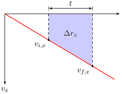
Fig. 6.2 \(x\) velocity vs. time graph for an object with a constant \(a_x\)

I know that \(a_x\) is constant, because the graph has a constant slope. To find the displacement, I need to find the area of the shaded region, defined by the time interval \(t\). Note that I am finding the exact area here, unlike in Lesson 04, since we assume we know the acceleration is constant. This can be divided into a rectangle and a triangle, so the area is

\[ \Delta r_x = v_{i, x} t + \frac{1}{2} (v_{f, x} - v_{i, x}) t = \frac{1}{2}(v_{i, x} + v_{f, x}) t \]

Performing the same derivation for the other two directions, I can write this as a vector equation, namely,

\[ \Delta {\vec r} = \frac{1}{2} ({\vec v}_i + {\vec v}_f) t \]

Problem

A flock of Canadian geese leave Newport for the winter, and head due south 150 km over the course of two hours. If their final velocity is 17.8 m/s southward and 4.92 m/s eastward, find the initial velocity of the geese (in m/s) at the beginning of the time period. Write your answer in unit vector notation, with \(+x\) pointing eastward, and \(+y\) pointing northward.

Answer: \({\vec v}_i = (-4.92 \textrm{ m/s}) {\hat x} + (59.5 \textrm{ m/s}) {\hat y}\)

Remember that the average velocity is defined as

\[ {\vec v}_{avg} = \frac{\Delta {\vec r}}{\Delta t} \]

so combining the last two equations gives (for constant acceleration)

\[ {\vec v}_{avg} = \frac{1}{2} ({\vec v}_i + {\vec v}_f) \]

Problem

Suppose you are given a graph of the \(x\) velocity vs. time for an object, as shown below. The acceleration is no longer constant, since the slope changes with time.

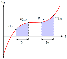
Fig. 6.3 \(x\) velocity vs. time graph for an object with changing \(a_x\)

1. If you use the above equation $\( \Delta {\vec r} = \frac{1}{2} ({\vec v}_i + {\vec v}_f) t \)\( to find the average velocity during time interval \)t_1\( (i.e. with initial and final velocities \)v_{1, x}\( and \)v_{2, x}$), would your answer be too big, too small, or exactly right?

2. What if you tried the same calculation for the average velocity during time interval \(t_2\), with initial and final velocities \(v_{3, x}\) and \(v_{4, x}\)?

Answer: Remember that the average velocity over a time interval is given by the displacement divided by the change in time. In particular, the displacement \(\Delta r_x\) in the \(x\) direction here is the area under the curve, so the question is whether using the “average area” equation

\[ \Delta r_x = \frac{1}{2} (v_{1, x} + v_{2, x}) t_1 \]

for the first interval, for example, is the right size. This is just the area of a trapezoid on its side, i.e. where its “height” is \(t_1\), and its two “bases” are \(v_{1, x}\) and \(v_{2, x}\). Thus, we need to see if this trapezoid matches the shaded areas. If you draw the appropriate lines to finish the trapezoids, you will see that the trapezoid is too small for time interval \(t_1\), and too large for \(t_2\). Thus, the “average” velocity calculated using the equation given above the problem is too small for the first interval, and too large for the second.

Problem

Why is the equation

\[ {\vec v}_{avg} = \frac{1}{2} ({\vec v}_i + {\vec v}_f) \]

incorrect with a non-constant acceleration? In other words, what goes wrong when the slope of the \(v_x\) vs. \(t\) graph is not constant?

Answer: The basic issue is that the equation assumes a constant rate of change from \({\vec v}_i\) to \({\vec v}_f\). For example, this means that the graph of \(v_x\) vs. \(t\) is a straight-line between \(v_{i, x}\) and \(v_{f, x}\). As you saw in the solution for the last problem, this can over- or underestimate the true displacement \(\Delta r_x\) if there is a non-constant acceleration.

To get our last vector kinematic equation, we can use our equation \({\vec v}_f = {\vec v}_i + {\vec a} t\) from above. Thinking in graph terms, this is the same as using the slope and the initial velocity to write down the final velocity. If we do this, then using \({\vec v}_f = {\vec v}_i + {\vec a} t\) along with our equation for \(\Delta {\vec r}\) from above gives

\[ \Delta {\vec r} = {\vec v}_i t + \frac{1}{2} {\vec a} t^2 \]

Problem

Write a vPython function calcDisp() that calculates the displacement of an object undergoing a constant acceleration over a given time. The arguments of this function are vPython vectors v_i and a, representing the initial velocity (in m/s) and acceleration (in m/s\(^2)\), respectively, and a scalar t giving the time interval (in s). The function should then return the displacement (in m) as a vPython vector.

Answer: Here is one solution to the problem; make sure you see what parts of the vector kinematic equation above match the vPython code below.

def calcDisp(v_i, a, t):
    '''
    Calculate the displacement of an object
    with a given initial velocity, and
    undergoing a constant acceleration over
    a time interval.
    '''

    return v_t * t + (1/2) * a * (t ** 2)

Problem

While coming in to land on a strange new planet, an astronaut has initial velocity of 8.75 m/s downward, 14.5 cm/s westward and 7.96 cm/s northward. After traveling for 2.15 minutes, the astronaut’s space vehicle lands on the planet. During this time, the lander’s vehicle had a displacement of 2.21 km westward, 1.18 km southward and 45.0 km downward. Find the acceleration of the lander (in m/s\(^2\)).

Answer: \({\vec a} = (-0.263 \textrm{ m/s}^2) {\hat x} + (-0.143 \textrm{ m/s}^2) {\hat y} + (-5.27 \textrm{ m/s}^2) {\hat z}\)

Problem

A sailboat is coasting on Narragansett Bay when the pilot realizes they are about to get hit by a large freighter. She turns on the boat’s motor, which accelerates the craft at 7.50 cm/s\(^2\) westward for 1/3rd of a minute. This moves the sailboat 50.0 m westward, and out of danger. What is the final velocity (in m/s) of the sailboat?

Answer: 3.25 m/s, westward

6.3. An example: free fall

As we saw in Lesson 05, a key case for one-dimensional motion is that of an object in a gravitational field. Obviously, this is something we deal with every day, so you should have some intuition about what results to expect. Let’s now go through such a problem, and see how the kinematic equations can be used to solve for quantities of interest. Consider the following.

Problem

A man, at the top of a 34.5 m tall cliff, throws a ball straight up with an initial velocity of 29.4 m/s.

1. How long (in s) does it take the ball to reach its maximum height?

2. How high (in m) is the maximum height above the ground?

3. How much time (in s)will it take for the ball to hit the ground?

4. What is the speed (in m/s) of the ball when it hits the ground at the bottom of the cliff?

If it is helpful, you can list your givens and unknowns in a table, as shown below. We are working in the vertical direction, so we use the \(y\) axis, with the \(+y\) direction pointing upwards. The subscript \(f\) is when the ball reaches the ground, while \(max\) is when the ball is at its maximum height. For convenience, we have made the ground to be \(r_y = 0.00\); then, when we calculate the maximum height above the ground, we do not have to add or subtract any extra number.

Quantity	\(y\)
\({\vec r}_i\)	34.5 m
\({\vec r}_{max}\)	? m
\({\vec r}_f\)	0.00 m
\({\vec v}_i\)	29.4 m/s
\({\vec v}_{max}\)	0.00 m/s
\({\vec v}_f\)	? m/s
\({\vec a}\)	\(-9.81\) m/s\(^2\)
\(t_{max}\)	? s
\(t_f\)	? s

Notice that the problem has a special position, known as the maximum height. This can be called the “peak”, the “highest point”, or other such terms. What is happening at this point is that the object stops moving upwards, and starts moving downward – it is turning around in the \(y\) direction. If you think about what this means, it requires the projectile to momentarily stop vertically. This is why the velocity \(v_{max, y} = 0.00\) m/s in the table.

So let’s start with finding the time to reach the maximum height, from its starting point. We have the vertical velocities at both of these points, and the vertical acceleration, so we can use

\[ v_{max, y} = v_{i, y} + a_y t_{max} \Rightarrow t_{max} = \frac{-v_{i, y}}{a_y} \]

since \(v_{max, y} = 0\). You may find it odd that there is a minus sign in front of the right-hand side of this equation. However, this is exactly what we need to get a positive time, since \(a_y < 0\). This is why you need to watch your signs when writing down your givens – if you choose them correctly, then in general, the calculation will automatically give you the right direction for your final answer. Plugging in the values from the test gives that \(t_{max} = 3.00\) s.

Next, we find how the maximum distance above the ground the ball reaches. Since all of the equations deal with displacement \(\Delta r_y\) from the initial point, then we can find this value, then use

\[ \Delta r_y = r_{max, y} - r_{i, y} \Rightarrow r_{max, y} = r_{i, y} + \Delta r_y \]

since all positions \(r_y\) are given in terms of the ground \(r_y = 0\). One way to solve this is using

\[ \Delta r_y = \frac{1}{2} (v_{i, y} + v_{max, y}) t_{max} \Rightarrow r_{max, y} = r_{i, y} + \frac{v_{i, y} t_{max}}{2} \]

Substituting into this last equation gives \(r_{max, y} = 78.6\) m.

We go through a similar process for finding the time to reach the ground, and the final velocity at that point.

When the motion ends

The velocity when an object hits the ground is not zero! If you think about why things stop when they hit the ground, it is because there is an extra acceleration (the “ground force”) acting. Remember you saw this in your graph of \(a_y\) vs. \(t\) at the end of Lesson 05. This is not included in the gravitational field, so we cannot use \(a_y = -g\) to solve for this. If it helps, think about questions like these as asking for the velocity (or time, or…) just before it hits the ground, when the motion is entirely due to only the gravitational field.

To find the time to reach the ground, without knowing the final velocity, I can start with

\[ \Delta r_y = v_{i, y} t + \frac{1}{2} a_y t^2 \]

However, there are two terms which have a time \(t\) in them, so it is not a simple matter of solving for one of these terms, and then dividing; this method will not have a time only on one side of the equation, but both! Thus, you need something slightly more sophisticated – here, you need to use the quadratic formula. Thus, you need to get the equation above into the standard form

\[ 0 = \frac{1}{2} a_y t^2 + v_{i, y} t - \Delta r_y \]

and then solve for \(t\). This gives

\[ t = \frac{-v_{i, y} \pm \sqrt{v_{i, y} ^2 + 2 a_y \Delta r_y}}{a_y} \]

Now, there is one last step, to write out \(\Delta r_y\) in terms of \(r_{i, y}\) and \(r_{f, y}\):

\[ t = \frac{-v_{i, y} \pm \sqrt{v_{i, y} ^2 + 2 a_y (r_{f, y} - r_{i, y})}}{a_y} \]

Notice this means \(\Delta r_y < 0\)! If you used the height of 39.4 m when substituting in for \(\Delta r_y\), you would get a different answer. It is important to watch your signs! When you put everything in correctly, you should get \(t_f = 7.00\) s.

Work in one step

Notice that we don’t have to “break up” the motion into pieces! We can find the total time of flight, without worry about how long it takes to get to the highest point, for example. It is much simpler to do it this way, and the physics equations “know” what the one, true trajectory is for the ball.

Finally, knowing as much as we do now, there are several choices for getting the final vertical velocity. Let’s stay simple, and use

\[ v_{f, y} = v_{i, y} + a_y t_f \]

As noted before, if you put in your values with the correct signs, you automatically get a downward (negative) velocity of \(v_{f, y} = -39.3\) m/s. Since speed is the magnitude of the velocity, the ball’s speed if 39.3 m/s when it hits the ground.

However, there is one extra nugget we can get from this problem. Specifically, we can discover an additional set of kinematic equations. Although they may look like it, these next equations cannot be written as a single vector equation, but there is one for each of the three coordinate axes \(x, y\), and \(z\). I will call these the scalar kinematic equations.

Suppose we knew the final velocity of the ball in this problem, and wanted to find the time of flight. Taking the same equation we just used, but now solving for \(t_f\), we get

\[ t_f = \frac{v_{f, y} - v_{i, y}}{a_y} \]

This looks a lot like

\[ t_f = \frac{-v_{i, y} \pm \sqrt{v_{i, y} ^2 + 2 a_y (r_{f, y} - r_{i, y})}}{a_y} \]

These equations match up (and we don’t have to worry about the \(\pm\) sign) if

\[ v_{f, x} ^2 = v_{i, x} ^2 + 2 a_x \Delta r_x \]

Note these are the \(y\) components of the vector, not the magnitudes; the same idea works for the \(x\) and \(z\) components as well.

\[ v_{f, x} ^2 = v_{i, x} ^2 + 2 a_x \Delta r_x \qquad v_{f, z} ^2 = v_{i, z} ^2 + 2 a_z \Delta r_z \]

Problem

You are walking out the door of Ripley Hall when you realize you don’t have your cover. You see your roommate in your room window and yell up for them to throw your cover downward to you. Use the information given in the vertical velocity vs. time graph shown below to answer the following questions, and remember you know what the slope of this graph is!

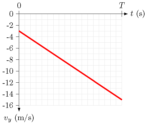
Fig. 6.4 Vertical velocity component vs. time for a falling cover

1. How long (is s) does it take for your cover to reach your hands? In other words, what is the value of \(T\)?

2. How high (in m) is your window above your hands?

3. Suppose your roommate instead threw your cover upward with a speed of 1.96 m/s. How long (in s) would it take to reach your hands now?

Answers: 1.22 s; 11.0 m; 1.77 s

6.4. Summary

This lesson expanded our mathematical tool kit to include the vector and scalar kinematic equations. For completeness, let’s list them all here.

\[ {\vec v}_f = {\vec v}_i + {\vec a} t \qquad \Delta {\vec r} = \frac{1}{2} ({\vec v}_i + {\vec v}_f) t \qquad \Delta {\vec r} = {\vec v}_i t + \frac{1}{2} {\vec a} t^2 \]

and

\[ v_{f, x} ^2 = v_{i, x} ^2 + 2 a_x \Delta r_x \qquad v_{f, y} ^2 = v_{i, y} ^2 + 2 a_y \Delta r_y \qquad v_{f, z} ^2 = v_{i, z} ^2 + 2 a_z \Delta r_z \]

These are exact when the acceleration of an object is constant. Even when the acceleration is not constant, these kinematic equations are the basis for everything we will be doing in computational physics. You have already seen how the first two allow us to update the position and velocity of a moving object. Later in the course, in Lesson 20, you will see how the last three provide a helpful window into the idea of work and energy. Understanding how to use these in various applications will be very important for you!

After this lesson, you should be able to:

• Explain when to use a particular vector or scalar kinematic equation

• Use the vector and scalar kinematic equations to solve a motion problem

5. Acceleration and free fall 7. Vector magnitude and direction