24. Coulomb’s law
24.1. Overview
Our current understanding of how physics works at a fundamental level is that there are four distinct interactions that explain all phenomena. Two of these operate only at the subatomic level, so we don’t have direct experience with them. These are the weak nuclear force – the reason that radioactive nuclei decay – and the strong nuclear force – which is why nuclei stay together the rest of the time! However, these forces act over distances of \(10^{-15}\) m or less, so we only see their effects only indirectly.
On the other hand, we will study two fundamental interactions that can act over any distance, because they are represented by inverse square laws. The first of these, gravitation, we looked at in Lesson 21. We now turn to the second, the electrostatic force, as given by Coulomb’s law. Much like gravity, the force between stationary electric chargess varies as \(1/r^2\). So while it does decrease with larger distance, the force never goes exactly to zero. However, unlike the masses of gravitation, electric charges come in positive and negative varieties. Thus, in most practical applications, the equal number of positive and negative charges in most matter reduces the size of the electrostatic force.
You may wonder why I keep using “electrostatic” as the name of the force, rather than “electric”. It turns out that when the electric charges are moving, the situation gets more complicated. First, a moving electric charge will create magnetic effects as well. However, the electric effects of the charge do not go away! To treat problems like this properly, one needs to combine both electricity and magnetism into an electromagnetic effect. It was James Clerk Maxwell, a Scottish physicist, who first worked out how to do so towards the end of the 19th century. So, I should really be calling this fundamental interaction “eletromagnetism”, rather than splitting off the electrostatic force by itself. However, treating elecromagnetism as a whole makes it more complicated! For now, we look at the simpler case of stationary electric charges.
Here are the objectives for this lesson:
State Coulomb’s law.
State the direction of the electrostatic force on a charge to due to like or opposite charges.
Given a situation with two or more charges, find the electrostatic force on each of the charges.
24.2. Electric charge
When we talked about the universal law of gravitation, we saw that there were two different types of constants involved:
The constant \(G\) gives the strength of the gravitational interaction between any two masses in the Universe. Making this number bigger or smaller would change the force of gravity between all pairs of objects exactly the same.
For a given object, its mass \(m\) describes how it is affected by the gravitational fields of all other objects. Unlike \(G\), we can change the mass of a single object, without affecting the masses of any other objects. Changing the mass of an object only changes the magnitude of the gravitational force on it.
When we talk about the electrostatic force, we will see this same type of structure. For now, let’s just focus on the electric analogue of the mass. This is known as the charge of an object. The charge \(q\) of an object is a measure of how that object is affected by the electrostatic force on the object, due to all other charges. Charge has units of coulombs (C).
As far as we can tell, all charges in the universe are multiples of a single value, \(e\), where
This is a magnitude of charge, so it means that a proton has a charge \(+e\), while an electron has a charge \(-e\). Thus, the size of a coulomb’s worth of charge is actually a large number of electrons; 1.00 C of charge is the charge of \(1/e = 6.22 \times 10^{18}\) electrons. The average lightning bolt has about a few tens of coulombs of charge. So, unlike the kilogram, the coulomb is actually a large unit!
Problem
A system is made of exactly 1525 particles, each of which is either a proton or an electron. If the net charge of the system is \(-5.456 \times 10^{-17}\) C, how many electrons are in this system? Hint: Write down two equations for the number of electrons \(n_e\) and protons \(n_p\) in the system, in terms of the total number \(N\) of particles and the total charge \(Q\), then solve for \(n_e\).
Answer: 933 electrons
The fact that all observable particles in the Universe have a charge that is an integer multiple of \(e\) is known as charge quantization. This is not an obvious fact, and it is unknown why it is true, although physicists have a few ideas.
24.3. Coulomb’s law
The equation for the electrostatic force is known as Coulomb’s law, and is in a similar form to that of Newton’s law of universal gravitation. We will again use the unit vectors \({\hat r}_{ij}\) as in Lesson 21, now defined based on the positions of the interacting charges \(q_i\) and \(q_j\). Remember we start from the relative position vectors,
and then define the unit vectors \({\hat r}_{ij}\) as
Each unit vector \({\hat r}_{ij}\) has its tail at object \(i\), and pointing away from object \(j\). This is shown in the diagram below, along with the position vectors, locating each charge relative to the origin. The unit vectors will give the line along which the electrostatic force points. Depending on the values of the charges \(q_i\) and \(q_j\), the force may point in the same direction as \({\hat r}_{ij}\), or in the opposite direction.
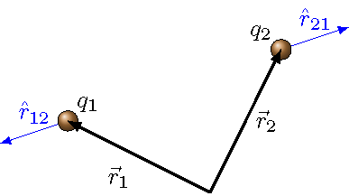
Fig. 24.1 The unit vectors \({\hat r}_{ij}\)
Let’s now get into the force equation. The electrostatic force on charge \(q_i\) due to charge \(q_j\) a distance \(r_{ij}\) away is stated mathematically as
with the constant \(k = 8.99 \times 10^9\) N\(\cdot\)m\(^2\)/C\(^2\).
The direction of the electrostatic force
There is no minus sign out in front, unlike the gravitational force equation! The minus sign in front of the gravitational force equation meant that force was always attractive, since the masses were positive. Here with Coulomb’s law, the direction of the electrostatic force is determined by the product of the charges. If \(q_i q_j < 0\), then the force is attractive. This gives the same overall minus sign we had with the gravitational force. If the product \(q_i q_j\) > 0 (i.e. both positive or both negative charges), then the force is repulsive. The force on the charge \(q_i\) points in the same direction as \({\hat r}_{ij}\), i.e. away from the other charge \(q_j\).
Here are some other properties of note. As with the universal law of gravitation, the electrostatic force also obeys Newton’s third law – if you flip the locations of the labels \(i\) and \(j\) in the equation, you get the same magnitude, just the opposite direction (since \({\hat r}_{ji} = -{\hat r}_{ij}\)). In addition, Coulomb’s law is also an inverse-square law, depending on the distance \(r_{ij}\) between the charges as \(1/r_{ij} ^2\).
You can experiment with the magnitude and direction of the electrostatic force, using the PhET application “Coulomb’s Law”. Clicking on “Macro Scale” uses distances of centimeters, and charges of microcoulombs; “Atomic Scale” uses distances of picometers and charges in multiples of \(e\).
Problem
Two identical point charges in free space are connected by a string 7.60 cm long. The tension in the string is 210. mN. What is the magnitude of the charge (in nC) on each of the point charges?
Answer: 367 nC
Problem
At what separation (in m) does the electrostatic force between \(+11.2\ \mu\)C and \(+29.1\ \mu\)C point charges have a magnitude of 1.57 N?
Answer: 1.37 m
24.3.1. Example: Return of the equilateral triangle
In Lesson 21, there was an example of the gravitational force on a mass at one corner of an equilateral triangle, due to masses at the other two corners. Let’s use the same triangle, but put charges on each of the particles. Then we will find the net electrostatic force on one of the charges. In some ways, this will be the same process as what we did with gravitation, but the effect of the charges will have an influence as well. I have used both positive and negative charges in this example, so you see how this affects the forces.
In the figure below, three charges are held in place at the corners of an equilateral triangle, again with sides \(d\) of 7.00 m. Here, we use charges \(q_1 = +2.00 \ \mu C\), \(q_2 = -4.00 \ \mu C\), and \(q_3 = +3.00 \ \mu C\). Note that the relative sizes of these charges are the same as the masses in the gravitation example of Lesson 21; however, we have changed the units from kg to \(\mu C\), and added in both positive and negative signs! Notice that I use the color coding of red as positive, and green as negative. We will now find the net electrostatic force on \(q_1\).
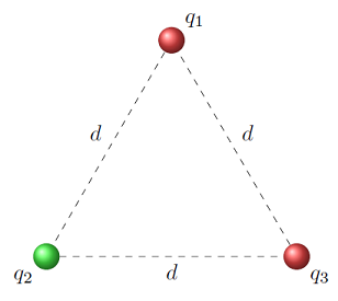
Fig. 24.2 Three charges fixed at the corners of an equilateral triangle
Notice that, because the geometry of the problem is the same as before, the unit vectors \({\hat r}_{12}\) and \({\hat r}_{13}\) are exactly the same as the previous example. The \({\hat r}_{ij}\) will always be the same, regardless of whether you are working with gravitational or electrostatic forces. Remember these unit vectors have a tail at the object of interest, and point away from the object exerting a force on it.
where \(\theta = 60.0^\circ\). When these are drawn, they look like the figure below – \({\hat r}_{12}\) is in the first quadrant, while \({\hat r}_{13}\) is in the second.
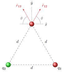
Fig. 24.3 Unit vectors \({\hat r}_{12}\) and \({\hat r}_{13}\)
However, the directions of the actual forces are not the same as the gravitational case, because of the signs of the charges. In particular, \(q_1\) and \(q_3\) will repel each other, since they are both positive, while \(q_1\) and \(q_2\) will attract each other, due to their opposite signs. This gives a different FBD that the gravitation example, so the signs of the charges \(q_i\) make a difference.
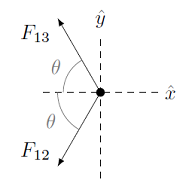
Fig. 24.4 FBD for charge \(q_1\)
Remember that we only care about the forces acting on \(q_1\); in particular, the force between \(q_2\) and \(q_3\) is irrelevant for what we are trying to do here. Remember Newton’s zeroth law!
Getting back to our problem, why do we have this difference between the directions of the unit vectors \({\hat r}_{12}, {\hat r}_{13}\) and the forces \({\vec F}_{12}, {\vec F}_{13}\)? Let’s work out what is happening for each force vector. The electrostatic force between charges \(q_1\) and \(q_2\) is given by
On the face of it, this force is in the first quadrant. However, remember that \(q_1\) and \(q_2\) are of opposite signs, so that the product \(q_1 q_2 < 0\). Thus, this vector is actually in the third quadrant, matching our FBD! Thus, this vector points in the second quadrant. Unlike the gravitational case, the number inside the parentheses is not always positive, so it can change the direction of the electrostatic force. The situation is different for \({\vec F}_{13}\), where
Here, \(q_1\) and \(q_3\) have the same signs, so that \(q_1 q_3 > 0\). If we compute the individual force vectors, we have that
and
Notice that the force components are much larger than those for the gravitational example, even though the charges “look smaller” than the masses did. The electrostatic force between two charges with roughly a coulomb of charge is much greater than the gravitational force between two kilogram-size masses. This is a result of the large size difference between the Coulomb constant \(k\) and the gravitational constant \(G\). Finding the total force gives
Using the Pythagorean theorem and the inverse tangent, this force has a magnitude of 1.32 mN and a direction of 194\(^\circ\) CCW from \(+x\) axis.
It is interesting to see how the direction has changed, relative to the gravitational example of Lesson 21. In that problem, since \(m_1\) is attracted to both \(m_2\) and \(m_3\), the net gravitational force on \(m_1\) was towards them, more or less along the \(-y\) axis. Here, though, \(q_1\) is repelled by \(q_3\), even though it is attracted to \(q_2\). Thus, the net force is roughly along the \(-x\) axis. The fact that the net electrostatic force includes both attraction and repulsion gives more variety in the magnitude and direction.
Problem
Using the same situation as above, find the net electrostatic force on \(q_3\).
Answer: \({\vec F}_3 = (-1.651 \times 10^{-3} \textrm{ N}) {\hat x} + (-9.533 \times 10^{-4} \textrm{ N}) {\hat y}\)
Problem
Write a vPython function netElectroForce() that finds the net electrostatic force on a charge, due to a collection of other charges. The arguments of this function should be the charge obj, and the list objList, a list of sphere objects with pos and charge attributes. Notice this is just the electrostatic version of the example program in Lesson 21, so you can use that program for guidance. Check the accuracy of your program by verifying the net forces on \(q_1\) and \(q_3\), as shown above.
Answer: Here is a sample program to solve the problem. The additional code at the end is what is needed to define the charges, and then find the net electrostatic force on \(q_1\).
def netElectroForce(obj, objList):

    # Definitions

    k = 8.99E9                    # Coulomb's constant (N m^2 / kg^2)
    netForce = vector(0, 0, 0)    # Initialize net force

    # Go through objects in objList, and
    # add its contribution to the net
    # electrostatic force on obj

    for otherObj in objList:

        # Find relation position vector r_ij

        rVec = obj.pos - otherObj.pos

        # Find unit vector, distance between charges

        rHat = hat(rVec)
        r = mag(rVec)

        # Find each electrostatic force vector

        netForce += (k * obj.charge * otherObj.charge / r ** 2) * rHat

    # Return final net force vector

    return netForce

# Definitions

d = 7.00                 # Triangle sides (m)
Q = radians(60)          # Triangle angles (rad)

# Create charges

q1 = sphere(pos = d * vector(-cos(Q), sin(Q), 0), \
            charge = 2E-6, color = color.red, \
            radius = 0.3)
q2 = sphere(pos = vector(-d, 0, 0), charge = -4E-6, \
            color = color.green, radius = 0.3)
q3 = sphere(pos = vector(0, 0, 0), charge = 3E-6, \
            color = color.red, radius = 0.3)

# Find net force on q1, due to q2, q3

result = netElectroForce(q1, [q2, q3])
print('Net electrostatic force on q1 =', result, ' N')
Challenge
Create a procedure forceMagDir() that prints out the magnitude and direction of the net electrostatic force. This procedure should use the same arguments as netElectroForce(), and you can use that function to find the net force in unit vector form. You will need to test which quadrant the net force is in, to give the correct direction.
Answer: Here is one possible solution.
def forceMagDir(charge, chargeList):

    # Get net force in unit vector form

    forceResult = netElectroForce(charge, chargeList)

    # Find magnitude of net force, print it out

    print('Net force magnitude =', mag(forceResult), ' N')

    # Find direction by finding which quadrant
    # the net force is in, then finding appropriate
    # angle CCW from +x axis

    angle = degrees(atan(abs(forceResult.y / forceResult.x)))

    if forceResult.x >= 0 and forceResult.y >= 0:
        print('Net force dir. =', angle, ' deg CCW from +x axis')

    if forceResult.x < 0 and forceResult.y >= 0:
        print('Net force dir. =', 180 - angle, ' deg CCW from +x axis')

    if forceResult.x < 0 and forceResult.y < 0:
        print('Net force dir. =', 180 + angle, ' deg CCW from +x axis')

    if forceResult.x >= 0 and forceResult.y < 0:
        print('Net force dir. =', 360 - angle, ' deg CCW from +x axis')
24.4. Summary
We have now discussed two of the long-range fundamental forces in the Universe: gravitation and the electrostatic force. They are similar in form and both rely on the unit vectors \({\hat r}_{ij}\). However, there is an important difference between the possible directions of the two forces, due to the positive and negative signs of electric charges, as opposed to mass always being positive. The force of gravity is always attractive, while the electrostatic force can be repulsive or attractive.
After this lesson, you should be able to:
State the value of \(e\).
Calculate the electrostatic force on a charge due to surrounding charges.