22. Gravitational potential energy
22.1. Overview
Link to the program in this lesson:
In Lesson 20 (conservation of energy), we used the form \(U_g = mgr_y\) for the gravitational potential energy of an object. However, this was based on a constant gravitational field, which works well when we are close to the surface of the Earth. Yet when we make more significant changes to our distance from the Earth, this is no longer a good approximation. It certainly will not be true when we start looking at orbiting objects! So, let’s see if we can find a more general form. This will allow us to use the techniques of conservation of energy for scenarios where there are significant changes in the gravitational field – for example, when a rocket is launched from the surface of the Earth. By the end of this lesson, we will find the escape speed necessary for such a rocket to avoid crashing back down to the Earth.
Here are the objectives for this lesson:
Define gravitational potential energy.
Identify the reference radius for zero gravitational potential energy.
Calculate the escape speed necessary to travel very far away from an object.
22.2. Gravitational potential energy
Let’s go back a step and recall the definition of the potential energy for any conservative force. In particular, the change in potential energy \(U_F\) for a conservative force \({\vec F}\), over a small interval \(\Delta {\vec r}\), is related to the work \(W_F\) done by that conservative force \({\vec F}\) over the same interval by the relation
In particular for gravity, suppose we move an object a distance \(\Delta r\) away from the Earth. This gives a displacement of \(\Delta {\vec r} = (\Delta r) {\hat r}\), where we are using the unit vector \({\hat r}\) at the object, pointing away from the Earth. On the other hand, as we just saw in Lesson 21, we can write the gravitational force as
Here, \(M\) is the mass of the Earth, \(m\) of the object, and \(r\) is the distance between them; I also use the same \({\hat r}\) as I did with \(\Delta {\vec r}\). Thus, the change in gravitational potential energy over the displacement \(\Delta {\vec r}\) is
since \({\hat r} \cdot {\hat r} = 1\), by definition. This gives the change \(\Delta U_g\) in gravitational potential energy for the Earth-object system as the distance between their centers goes from \(r\) to \(r + \Delta r\).
To get a handle on how this is different than the \(mgr_y\) function we used before, the program below creates a graph for the two versions. The scenario is the following: a 1.00 kg mass is lifted from the surface of the Earth up to a height of 250. km above the surface. The red curve on the graph just shows \(mg(R_E + h)\), where \(R_E\) is the Earth’s radius, and \(h\) the altitude of the object above the surface. This is what the gravitational potential energy would be if we could assume a constant gravitational field \({\vec g}\) for all heights \(h\). On the other hand, the blue line adds up all of the \(\Delta U_g\) as the object moves, and shows the total up to that height \(h\). These \(\Delta U_g\) are computed over height intervals \(\Delta r\) of 10.0 m; you can see the specific code by clicking on the pencil icon of the app. Note that in both cases, since we are graphing \(\Delta U_g\) from the surface, then we have chosen our \(U_g\) such that \(U_g = 0\) at the surface; I will come back to this point later. Run the program, and see how the two functions compare. Notice that the values of \(U_g\) are given in megajoules (MJ), and height \(h\) in km.
Notice a few things about this graph. First, the definition \(mgr_y\) works really well up to about 100-150 km; you can’t the difference between it and the proper definition for these altitudes – the gravitational field within that height range is really close to 9.81 m/s\(^2\). If we climbed the highest mountains, we would barely even notice the change! This is why we have assumed the gravitational field is constant – for all applications we’ve dealt with so far, it basically stays the same. Notice that a lot of the intuition we have developed previously still works out. In particular, the gravitational potential energy of the Earth-object system increases as the two get further apart.
However, eventually the distance between the Earth and the object we are lifting up become significant. As we get further away from the Earth’s center, the gravitational field magnitude \(g\) gets smaller, so it takes a little less energy to raise the object a further 10.0 m at heights of 100. km and greater. Thus, the red and blue curves start to diverge, with the actual \(\Delta U_g\) a little smaller than the equation given by \(mgr_y\). This is because of the inverse square law nature of the gravitational force (\(1/r^2\) in the denominator).
Problem
Change the maximum height H_F in the code to something larger. What do you notice about the actual \(U_g\) curve? Try at least a value of 2000. km.
Let’s now go back to the issue of where to choose \(U_g = 0\). When using \(mgr_y\) near the surface, we had the freedom to choose our reference level \(r_y = 0\), i.e. the height where \(U_g = 0\). This is because we were assuming a constant gravitational field, so there was no natural altitude to use. For the general case, however, there is a natural distance \(r\) to use, although it may seem odd at first. Our definition of \(U_g\) will assume that \(U_g \to 0\) as \(r \to \infty\); in other words, \(U_g\) is zero when the two objects are “very far away” from each other. This situation is more like that of a spring, and elastic potential energy. In that case, there is a natural place for the reference, namely the equilibrium point \(r = 0\) where the spring is neither stretched nor compressed. Obviously, if the spring is at its equilbrium point, there is no energy stored in the spring, so it makes sense that \(U_{spr} = 0\) there.
This gives the following equation:
Quantity: gravitational potential energy
Symbol: \(U_g\)
Definition: For two masses \(m_i\) and \(m_j\) separated by a distance \(r_{ij}\), the gravitational potential energy is
SI units: joules (J)
This is a scalar quantity, not a vector
The minus sign is important in this definition, but again, it is probably strange the first time you see it. But it matches our intuition for how \(U_g\) changes with distance. If I throw a ball up in the air, the gravitational potential energy of the ball-Earth system increases. But it’s just that this is because \(U_g\) goes from a larger negative number to a smaller one, not because it goes from a small positive number to a larger one.
Problem
A planet has an orbit around its parent star as shown below. At which point does the planet-star system have the greatest gravitational potential energy? Answer in terms of values along the number line.
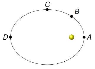
Fig. 22.1 A planet in orbit around its parent star
A
B
C
D
Answer: The conceptual idea is the same as when we looked at gravitational potential energy near the surface of the Earth (i.e. of the form \(mgr_y\)) – the further the two objects are apart, the bigger the value of \(U_g\) as a number. Thus, the largest \(U_g\) is when the planet is at point \(D\). At point \(D\), the gravitational potential energy \(U_g\) is negative, but the closest to \(U_g = 0\) out of all four points. At point \(A\), \(U_g\) is its most negative value, since \(r\) is the smallest, so it has the smallest \(U_g\) at this location.
I will return to this negative sign in Section 22.4, where the sign of \(U_g\) gives information about the properties of the system. First, however, let’s figure out how the different form of the gravitational potential energy changes the maximum height of an object going upward from the Earth’s surface.
22.3. Escape speed
One of the first topics we covered in this class, back in Lesson 05 (acceleration and free fall), was what happens when you throw a ball up into the air – how high does it go? Remember that this was using the assumption that the gravitational field was constant, as it is near the surface of the Earth. This field has very little variation over the heights we normally encounter during our daily routine.
But how would this change if something was moving very fast, and we had to worry about a decreasing gravitational field as we move away from the Earth? One way to do this would be to take into account the changing field. For example, you could write a Python program, where the position and velocity of the moving object is updated using an acceleration that depends on the height above the Earth’s surface.
However, this is really overkill, since the changing field is “taken into account” by the gravitational potential energy. All we really need to do is use is conservation of mechanical energy, using the \(U_g\) from this lesson, rather than the equation \(mgr_y\) (which assumes a fixed gravitational field \(g\)). Then we can find how high an object moves if it has some starting speed at ground level.
To show how this works, let’s go through the following example. The largest rocket ever built is the Saturn V, used to put US astronauts on the Moon. Suppose instead this \(2.97 \times 10^6\) kg rocket is launched from the surface of the Earth into deep space. The Earth has a mass of \(5.97 \times 10^{24}\) kg and a radius of 6,380 km; ignore the effect of the Sun and the other planets. We are going to find the necessary launch speed for the Saturn V to momentarily stop at the height of low Earth orbit (LEO), 2000 km away above the surface of the Earth.
We are ignoring the effects of air resistance on the rocket, so \(W_{NC} = 0\). Then we can use conservation of mechanical energy to solve for the final distance from the surface. At its launch, the rocket has both kinetic and gravitational potential energy; it starts at a distance \(r = R_E = 6380\) km from the Earth’s center with a speed \(v_i\), so its initial mechanical energy is
where \(M_E\) is the mass of the Earth, and \(m_S\) is the mass of the Saturn rocket. At the rocket’s highest point, it just reaches LEO, so its final speed \(v_f = 0\). This will be at a height \(h = 2000\) km above the surface, so it is a distance \(R_E + h\) away from the Earth’s center. This gives the final mechanical energy as
Setting these equal to each other, notice that the mass \(m_S\) is in every term, so it can be canceled out – the mass of the rocket doesn’t matter!
Ignoring the rocket mass
You may be a little uncomfortable about the fact we can get rid of the Saturn rocket’s mass. Does that mean we can make the rocket as big as we want, and it doesn’t matter? Well, no, because I am really assuming that the mass \(M_E\) of the Earth is much bigger than the mass \(m_S\) of the rocket. If this were not true (imagine a binary star system, with two stars the same mass), then the masses we use would be more like an “averaged” mass, much like what we did in Lesson 09 when we talked about the center of mass. This would be necessary in order to have conservation of linear momentum. In the case considered here, the masses we are using are essentially correct, and give a very small error, so I don’t worry about it.
Dividing out by the mass of the rocket, this gives the energy equation
The gravitational potential energy terms can be moved to the same side, then you can solve for \(v_i\). This gives
Plugging in the numbers from above, one finds the initial speed must be 5.46 km/s to just barely reach LEO.
Notice that we get a bonus by doing the algebra – we can now find the necessary speed to reach any distance \(h\) above the surface. In fact, we can figure out the speed needed to go “very far away”, in other words, when \(h \to \infty\). This gives the speed known as the escape speed \(v_{esc}\): the speed required to travel an infinite distance away from another object. In practice, this just means a large distance, compared to the size of the object left (for example, the Earth). Starting with our last equation, and taking the limit of \(h\) going to infinity, we have that
So the second term disappears, and the escape speed is
We can now easily calculate the escape speed for the Earth as 11.2 km/s.
Problem
The mass of the planet Mars is \(6.42 \times 10^{23}\) kg, and its radius is 3397 km. The larger of its two satellites, Phobos, orbits at a distance of 5979 km above the surface of Mars.
What is the necessary launch speed for the Saturn V to just reach Phobos’ orbital radius?
How fast would it have to leave Mars’ surface in order to travel very far away from the planet?
Answers: 4.01 km/s; 5.02 km/s
Problem
Write a vPython function maxLaunchAlt() that finds the maximum height reached above the surface of a planet, when an object is launched vertically with a given speed. The arguments of the function are M_P, the mass of the planet (in kg); R_P, the radius of the planet (in km); and v_i, the initial vertical velocity component of the object (in km/s). Assume that the object has a negligible mass, compared to the planet. The function should return the maximum altitude (in km) the object reaches, before stopping and falling back towards the planet.
Answer: First, you need to solve the energy equation above for \(h\) as a function of \(M_P, R_P\) and \(v_i\). When you do this, you should get
Below is a possible implementation of this algebraic equation in vPython.
def maxLaunchAlt(M_P, R_P, v_i):

    G = 6.67E-11        # Gravitational constant (N m^2 / kg^2)

    # Convert quantities to proper units

    R_P *= 1000         # R_P to meters
    v_i *= 1000         # v_i to m/s

    # Calculate final altitude h in meters

    h = 1 / (1 / R_P - v_i ** 2 / (2 * G * M_P)) - R_P

    # Return value in km

    return h / 1000
You can verify this program works by comparing it to the problems we did earlier. For example, maxLaunchAlt(5.97E24, 6380, 5.46) should give a result of 2000 km, while maxLaunchAlt(6.42E23, 3397, 4.01) should return the value 5980 km (both of these to three sig figs).
22.4. Energy graphs and gravitational potential energy
Now I will turn to a graphic method of thinking about the motion of escape speed. I will mirror the discussion above, where motion is only radial, i.e. there is no perpendicular velocity component \(v_\perp\); we will talk about the effective potential energy for gravity in the next lesson. Remember from the energy graphs section of Lesson 20 how plotting the mechanical energy of a system onto the potential energy graph will give an idea of how fast an object is moving, and at which points it will momentarily stop. In particular, the mechanical energy \(E\) will be a horizontal line, if there are no non-conservative forces such as air resistance or friction. Then the “gap” between this total energy, and the potential energy \(U\) of the system will be the kinetic energy \(K\). The larger this gap, the greater \(K\) will be, and therefore the larger the speed. On the other hand, if the mechanical and potential energy curves intersect, the kinetic energy is zero, and the system momentarily stops moving.
To apply this to a gravitational system, in the figure below, I have graphed two possible values for the mechanical energy \(E\) – one negative, and the other positive. We can interpret these in terms of the motion, as described above, and also to the escape speed we just finished discussing.
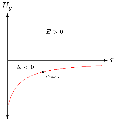
Fig. 22.2 Possible values of the mechanical energy \(E\), for a \(U_g\) vs. \(r\) graph
In particular, notice that the line with negative mechanical energy \(E < 0\) intersects the gravitational potential energy \(U_g\) curve at a distance \(r_{max}\). So, if the object is initially moving upward, it will slow down (smaller gap between \(E\) and \(U_g\)) until it reaches \(r_{max}\), then fall back downward, i.e. move in the direction of smaller \(r\). Since the mechanical energy is negative, the object does not have enough energy to escape; thus, situations where \(E < 0\) are known as bound systems.
On the other hand, when there is a positive mechanical energy \(E > 0\), there is always a non-zero gap, so the object keeps moving towards larger \(r\), even though it slows down as it does so. Even in the limit of infinite \(r\), it will have some kinetic energy, since \(U_g \le 0\) for all \(r\). This is an unbound system, with \(E > 0\).
The boundary between these two cases is exactly what we treated when we found the escape speed. Remember there, we wanted to “just barely” reach an infinite distance. This is what happens when we have \(E = 0\), with the stopping point of the object now at \(r = \infty\). Any speed above the escape speed gives \(E > 0\), while anything below has \(E < 0\), and a stopping point smaller than an infinite distance.
Notice that everything I have said here is true for a generic potential energy, where \(\lim_{r \to \infty} U(r) = 0\). Thus, it also works for the electrostatic potential energy of charged particles. In particular, you may have wondered why the electrons in an atom are said to have negative energy; the reason is the same as here, where the electrons are bound to the atomic system, and cannot escape without an input of energy from the outside. We will also see these graphical methods in the next lesson, when we turn to orbiting objects. Here, we only looked at motion towards or away from the gravitational center \({\vec r} = {\vec 0}\); in Lesson 23 (Kepler’s laws), we will consider how the picture changes when there is a motion around the center as well.
22.5. Summary
We now have all of the tools needed to understand the motion of objects in the Solar System. In Lesson 21, we discussed Newton’s law of universal gravitation; this is the interaction force between all bodies, large and small, moving around the Sun. Thinking about how this gravitational force provides a necessary centripetal force (Lesson 16) will allow us to start talking about the size of orbits, and the time needed to complete one.
In this lesson, we defined the gravitational potential energy, based on the gravitational force. Along with conservation of energy (Lesson 20), we can now relate the distance between the Earth and an orbiting satellite to its kinetic energy, and thus its speed. This will give us a relation between speed and distance. However, remember we also have conservation of angular momentum (Lesson 18), which relates distance and the perpendicular velocity component. Thus, between these two conservation principles, we can find the velocity of an orbiting object, given its distance away from a planet, because we can use the speed, along with the perpendicular velocity component, to find the radial velocity component.
This overview shows us all the physics tools that we can use to understand orbital motion. With this perspective, we next head to Lesson 23, and show how these all come together in Kepler’s laws of planetary motion.
After today’s class, you should be able to:
Calculate the gravitational potential energy of a system of masses
Find the escape speed for a given astronomical object